NPER Function in Excel

If you want to figure out how many payment periods it takes to pay off a loan, hit a savings goal, or drain a retirement account, the NPER function is what you’re looking for.

As long as the interest rate and payment amount stay constant, NPER gives you the count of periods that makes the math balance.

NPER returns a single value, but it works just fine inside dynamic array formulas like =NPER(B2:B8/12, -C2:C8, D2:D8) when you want to evaluate a whole column of scenarios in one shot.

In this article, I’ll walk you through the syntax, the sign convention that trips most people up, and a few practical examples.

NPER Syntax

Here is the syntax of the NPER function:

=NPER(rate, pmt, pv, [fv], [type])

• rate – The interest rate per period. If your loan has an annual rate but monthly payments, divide the annual rate by 12.
• pmt – The payment made each period. It stays the same across all periods. Enter outflows (money you pay) as negative numbers.
• pv – The present value, or the lump-sum amount the future payments are worth right now. For a loan, this is the amount you borrowed.
• fv – Optional. The cash balance you want left after the last payment. Defaults to 0 if you skip it, which is right for most loan scenarios.
• type – Optional. Set to 0 (or skip) if payments happen at the end of each period, or 1 if they’re at the beginning.

A quick heads-up on the sign convention. Excel treats money you pay out as negative and money you receive as positive.

So for a loan, the present value (the amount you borrowed) is positive and the payment is negative. For a savings plan, the payment is negative (you’re paying into the account) and the future value goes in as a positive number.

Flipping the signs feels weird the first few times, but it’s the same convention you’ll see across PV, FV, PMT, and RATE.

When to Use NPER Function in Excel

Use this function when you need to:

• Figure out how many months or years it takes to pay off a loan at a fixed payment
• Calculate how long it takes to reach a savings goal at a fixed contribution
• Estimate how many years a retirement balance lasts at a fixed withdrawal rate
• Compare two payment plans by how long each one runs
• Run what-if scenarios across a column of different payment amounts in one formula

Let me show you a few practical examples so the function actually clicks.

Example 1: Months to Pay Off a Personal Loan

Let’s start with the most common case.

Below is the dataset. You borrowed $18,500 for a kitchen renovation at a 9.25% annual interest rate, and you’re paying $325 a month.

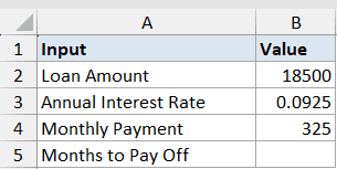
I want to know how many monthly payments it takes to pay this off completely.

Here is the formula:

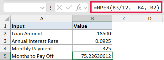
=NPER(B3/12, -B4, B2)

How this formula works:

• B3/12 converts the 9.25% annual rate into a monthly rate, because payments are monthly.
• -B4 is the monthly payment of $325, entered as negative since it’s money going out.
• B2 is the $18,500 loan balance, entered as positive since you received that amount.

The result comes back around 73.2 months, so roughly 6 years and 1 month to clear the loan. The decimal means the last payment will be smaller than $325, since you don’t owe a full payment for that final fraction.

Pro Tip: If you only want whole months (since you can’t really make a partial payment), wrap NPER in ROUNDUP: =ROUNDUP(NPER(B3/12, -B4, B2), 0). That gives you 74, which is what a loan amortization schedule will actually show.

Example 2: Years to Hit a Down-Payment Savings Goal

Here’s a scenario most people will recognize.

Below is the dataset. You’re saving for a $60,000 house down payment. You already have $8,000 set aside, you can contribute $750 every month, and the account earns 4.5% annually.

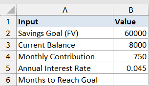
I want the number of months it takes for the account to grow from $8,000 to $60,000.

Here is the formula:

=NPER(B5/12, -B4, -B3, B2)

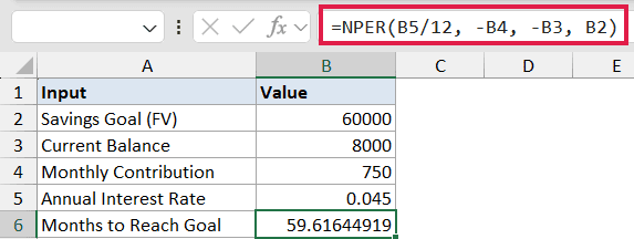
In the above formula, the rate is divided by 12 to match the monthly contributions. Both the starting balance and the monthly payment are entered as negative because they represent money leaving your pocket and going into the account.

The future value of $60,000 is positive since that’s the amount you’ll have at the end.

The result is about 53.6 months, or just under 4 and a half years.

If you want to know how many years instead of months, divide by 12: =NPER(B5/12, -B4, -B3, B2)/12.

If you’re more interested in how the balance grows than in the time-to-goal, the compound interest formula approach gives you the year-by-year balance trail.

Example 3: How Long a Retirement Balance Lasts

Now let’s flip the question. Instead of saving up, you’re drawing down.

Below is the dataset. A retiree has $480,000 saved, the account earns 4% annually, and they plan to withdraw $3,500 a month.

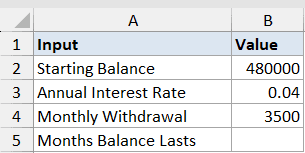
I want the number of months the balance will last before it hits zero.

Here is the formula:

=NPER(B3/12, B4, -B2)

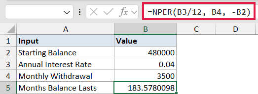
Notice the sign flip here. The starting balance of $480,000 is negative because from Excel’s perspective it’s money currently parked in the account. The $3,500 monthly withdrawal is positive because it’s coming back to the retiree as income.

The result is roughly 207 months, or about 17 years and 3 months at this withdrawal rate.

Caveat: NPER returns #NUM! when the math is impossible. If the withdrawal is so small that the interest earned each month exceeds it, the account never depletes and NPER throws an error.

For example, dropping the withdrawal to $1,500 a month at this rate gives #NUM! because $480,000 at 4% earns $1,600 a month in interest alone.

If the withdrawal itself grows over time (say, with inflation), look at a growing annuity instead, because NPER assumes constant payments.

Example 4: Scenario Sweep With Different Payment Amounts

This is where NPER’s composition with dynamic arrays comes in handy.

Below is the dataset. You’re shopping for a $25,000 car loan at 6.75% APR and want to see how the payoff timeline shifts as you change the monthly payment. The column has seven payment amounts to try, from $400 up to $750.

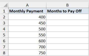
I want to fill the Months to Pay Off column for every payment scenario in one go.

Here is the formula:

=NPER(0.0675/12, -A2:A8, 25000)

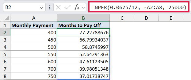
NPER itself returns a single value per call, but when you feed it an array (the column of payment amounts in A2:A8), Excel 365 evaluates it row by row and spills the results down. One formula fills all seven rows.

A $400 payment takes around 77 months to clear the loan. A $750 payment cuts that to about 38 months.

Doubling the payment doesn’t halve the time exactly because the higher payments knock down the principal (and therefore the interest) faster.

If you’re on Excel 2019 or older, this won’t spill. Drop =NPER(0.0675/12, -A2, 25000) in B2 and drag it down.

Caveat: The array length matters. If one column has 7 values and another has 5, NPER returns #N/A past row 5. Either trim the arrays to the same length, or use a structured table reference so they grow together.

Example 5: End of Period vs Beginning of Period

This one’s about a quiet detail that changes the answer more than people expect.

Below is the dataset. You’re investing $500 a month into an account earning 6% annually, with a target balance of $100,000.

The question is whether you deposit at the start of each month or at the end.

I want to compare the number of months it takes under each timing.

Here are the formulas:

=NPER(B2/12, -B3, 0, B4, 0)

=NPER(B2/12, -B3, 0, B4, 1)

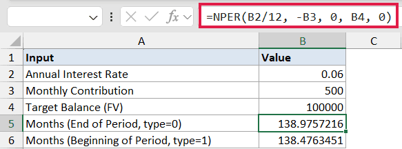
The only difference between the two formulas is the last argument. A 0 means deposits land at the end of the month. A 1 means they land at the beginning, so each deposit earns one extra month of interest before the next one comes in.

End-of-period comes out to roughly 138 months. Beginning-of-period comes out to about 137 months.

The gap is small on a 10-ish-year horizon, but it widens as the timeline gets longer. On a 30-year retirement account, the same flip can shave close to a full year off the answer.

The same type argument behaves the same way in PV, FV, PMT, and RATE. If you’re matching NPER’s output against a payment schedule from a bank or a brokerage, check which timing they use.

Most US mortgages use end-of-period. Most leases and rent payments use beginning-of-period.

Tips & Common Mistakes

• Mind the sign convention. For a loan, present value is positive and payment is negative. For a savings plan, both the starting balance and the payment are negative, and the future value is positive. Getting one sign wrong is the most common NPER mistake.
• Match the rate to the period. Annual rate with monthly payments means dividing the rate by 12. Quarterly payments means dividing by 4. Forgetting this is the second most common mistake.
• #NUM! usually means the math is impossible. It shows up when the payment is too small to cover the interest charged each period, or when the target future value can never be reached at the given rate and payment. Increase the payment or check the sign of one of the inputs.
• Use ROUNDUP for practical period counts. NPER gives you a decimal like 73.2 months, but you can’t make 0.2 of a payment in the real world. =ROUNDUP(NPER(...), 0) gives you the actual month count that the lender’s amortization schedule will show.
• Don’t forget the optional arguments. Skipping fv is fine for vanilla loans (where the goal is to pay it off to zero). But for savings plans, retirement drawdowns, or balloon-payment loans, fv has to be set or the answer is wrong.
• NPER assumes constant payments. If your cash flows vary period to period, NPER is not the right tool. Look at NPV or IRR for irregular cash flow series instead.
• The whole family works together. If you know any four of (rate, nper, pmt, pv, fv), you can solve for the fifth using PV, FV, PMT, RATE, or NPER. They all share the same sign convention, so once it clicks for one, it clicks for all of them.

NPER is the function you reach for when the question is “how long?” It sits behind most loan-payoff and savings-goal calculators you’ll come across.

The hardest part is the sign convention. Once that clicks, the rest is just plugging numbers into the right slots.

Try it on a real number you’re tracking, like a car loan you’re paying down or a savings account you’re trying to fill. Seeing the period count sit next to the headline payment often changes how the deal looks.

List of All Excel Functions