PI Function in Excel

If you need the value of pi for a circle or any geometry calculation in Excel, the PI function gives it to you with full precision. You don’t have to type out 3.14159 and worry about how many digits to include.

PI does not spill on its own. It returns a single value per call, but it composes cleanly inside array math. In this article, I’ll show you how to use PI to find circumference, area, convert degrees to radians, and feed an array formula.

PI Function Syntax in Excel

The PI function takes no arguments at all. You just call it with empty parentheses.

=PI()

It returns the constant 3.14159265358979 (15 significant digits). There are several ways to use pi in Excel, but the function is the cleanest. There are no arguments to pass, but the parentheses are still required.

When to Use PI Function

Here are some common situations where PI comes in handy:

• Calculating the circumference of a circle from its radius or diameter.
• Calculating the area of a circle, a sector, or an ellipse.
• Converting angles between degrees and radians for trig functions.
• Finding the volume or surface area of cylinders, spheres, and cones.
• Any formula where you’d otherwise hard-code 3.14159 and lose precision.

Example 1: Find the Circumference of a Circle

Let’s start with a simple example.

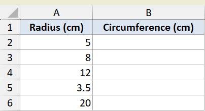
Below is the dataset with a list of circle radii in column A and an empty Circumference column in B.

I want to find the circumference of each circle, which is 2 times pi times the radius.

Here is the formula:

=2*PI()*A2

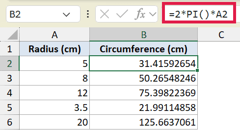
For a radius of 5 cm, this returns 31.4159, which is 2 times 3.14159 times 5. Copy the formula down column B and every radius gets its circumference.

Using PI() here keeps all 15 digits of precision, so your results stay accurate no matter how big the radius gets.

Example 2: Calculate the Area of a Circle

Here’s another practical scenario.

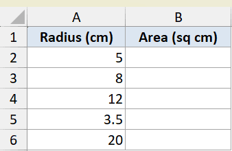
Below is the same set of radii, this time with an Area column waiting to be filled.

I want the area of each circle, which is pi times the radius squared.

Here is the formula:

=PI()*A2^2

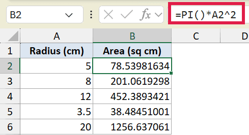
For a radius of 5 cm, this returns 78.5398, which is 3.14159 times 25. The ^ is the exponent operator, so A2^2 squares the radius before multiplying by pi.

Note that Excel applies the exponent before the multiplication, so you don’t need extra parentheses around A2^2 here.

Example 3: Convert Degrees to Radians

Let’s look at a common trig setup.

Below is a list of angles in degrees in column A, with a radians column to fill.

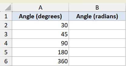
I want to convert each angle from degrees to radians, which means multiplying by pi and dividing by 180.

Here is the formula:

=A2*PI()/180

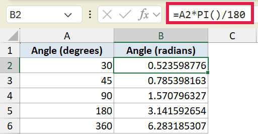
For 30 degrees, this returns 0.5236 radians. Excel’s trig functions like SIN and COS expect radians, so this conversion is something you’ll do often.

Pro Tip: Excel has a dedicated RADIANS function that does this directly. You can write =RADIANS(A2) instead of =A2*PI()/180 and get the same result with less typing. DEGREES(A2) is the reverse, for turning radians back into degrees.

Example 4: Use PI Inside a Spilling Array Formula

Let’s step it up with a single formula that handles a whole table at once.

Below is a dataset with cylinder radii in column A, heights in column B, and an empty Volume column in C.

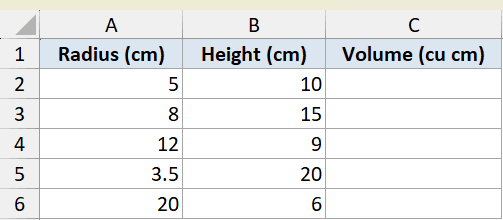
I want the volume of each cylinder, which is pi times the radius squared times the height. I’ll do all five rows with one formula.

Here is the formula:

=PI()*A2:A6^2*B2:B6

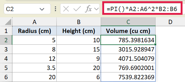
Enter this in C2 and the result spills down to C6 automatically. The first cylinder returns 785.398 cubic cm.

What makes this spill is the ranges A2:A6 and B2:B6, not PI() itself. PI() returns its single constant, and Excel applies it across every row of the array.

This is the cleanest way to see PI work inside a 365 array formula. There’s no copying down, just one formula doing the whole column.

Tips & Common Mistakes

• Don’t forget the empty parentheses. Typing =PI returns a name error. PI is a function, so it always needs =PI() with the parentheses, even though there’s nothing to put inside them.
• Use PI() instead of typing 3.14159. Hand-typing the value truncates the precision and can throw off results in long chains of math. PI() always carries 15 digits, and you can always round the final answer to the decimals you need.
• Use RADIANS and DEGREES for angle conversions. Instead of =angle*PI()/180, the RADIANS function does the degrees-to-radians step directly, and DEGREES does the reverse.
• Watch the exponent order. In a formula like =PI()*A2^2, Excel squares A2 first, then multiplies by pi. If you ever want to square the whole product, wrap it in parentheses.

PI is one of those small functions you’ll reach for constantly once you start doing any geometry or trig in Excel. It hands you a precise constant with zero arguments, and it drops right into bigger formulas, including array formulas that fill a whole column at once.

Once you’re comfortable with it, pairing PI with RADIANS, DEGREES, and the trig functions covers just about every circle and angle calculation you’ll run into. If you work with the other math constant, the EXP function gives you e raised to a power the same precise way.

List of All Excel Functions

Related Excel Functions / Articles:

• LN Function in Excel
• Microsoft Excel Terminology (Glossary)
• How to Use ‘e’ in Excel? (Euler’s Number)
• How to Square a Number in Excel?