
If you want to show the less than or equal to sign (≤) in Excel, you’ve probably noticed there’s no key for it on your keyboard.
There are a few ways to get it into a cell, from a keyboard code to a dialog box to a formula. I’ll walk you through five of them.
One thing worth clearing up first. If you want Excel to actually compare values, this glyph won’t do it. Excel uses <= for that, typed as two separate characters, exactly the way the greater than or equal to operator uses >=.
Method #1: Using the Alt Code
The quickest route on Windows is the Alt code. You hold the Alt key, type a number on the numeric keypad, and the ≤ character drops straight into the cell.
Below I have a discount tier table. I want the Order Quantity column to read “≤ 50” instead of spelling out “50 or less.”
Here are the steps to insert the ≤ sign using its Alt code:
- Double-click the cell where you want the ≤ sign, and put the cursor where the symbol should go.
- Make sure Num Lock is on, then hold the Alt key and type 243 on the numeric keypad.
- Release the Alt key. The ≤ symbol appears in the cell. Press Enter to confirm.
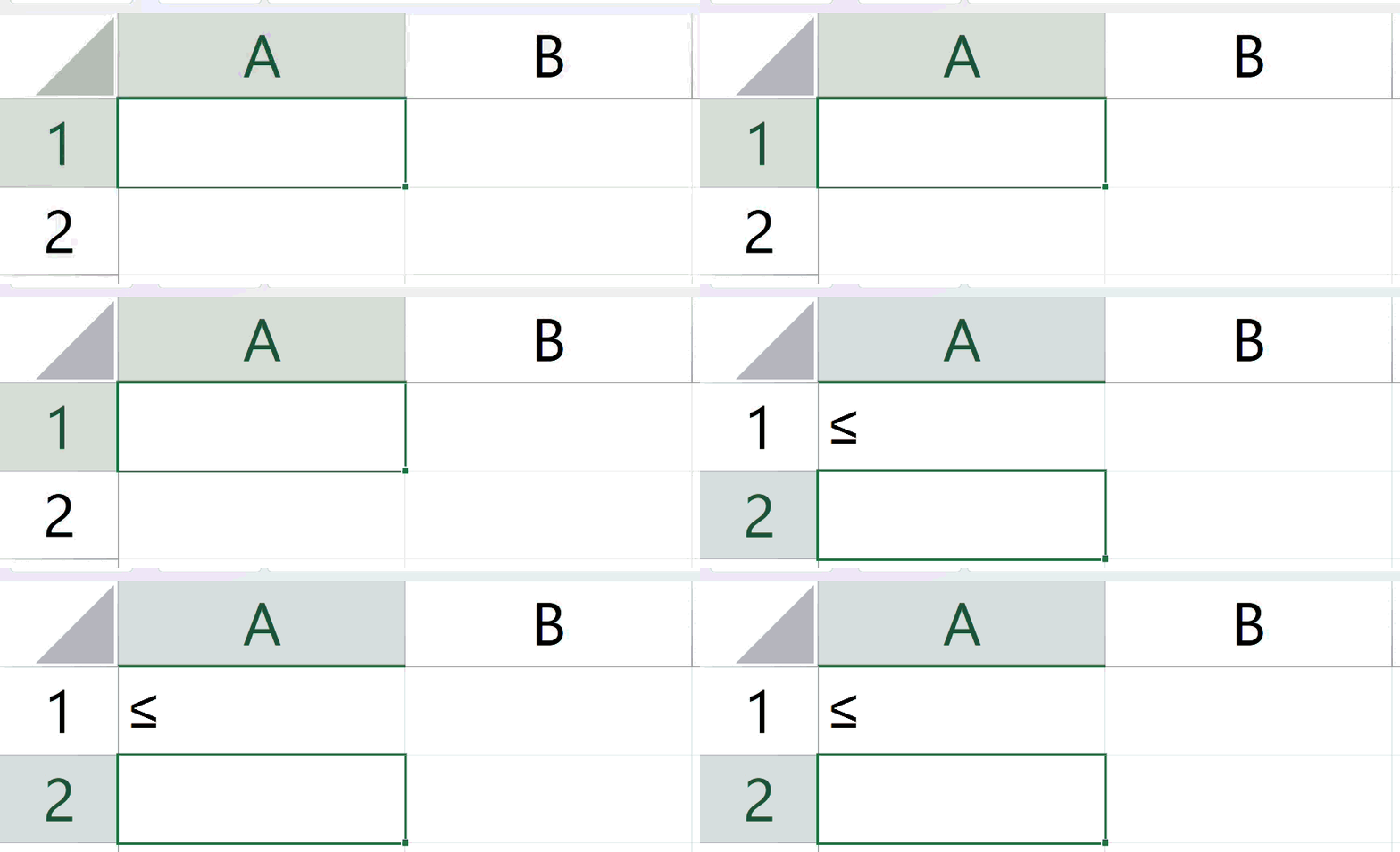
Use the numbers on the numeric keypad, not the row of numbers above the letters. Those top-row keys won’t produce the symbol.
Note: Alt + 243 reads from your system’s OEM code page, which is CP437 on most English Windows setups. If you get a different character, or you are on a laptop with no numeric keypad, use the Symbol dialog box in Method #2. On a Mac, press Option + comma (,) to type ≤ directly.
Method #2: Using the Symbol Dialog Box
If you’d rather not memorize a code, the Symbol dialog box lets you browse for the ≤ sign and click to insert it. The steps below are for Excel on Windows.
Here are the steps to insert the ≤ sign from the Symbol dialog box:
- Click the cell where you want the ≤ sign.
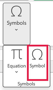
- On the Insert tab, in the Symbols group, click Symbol.
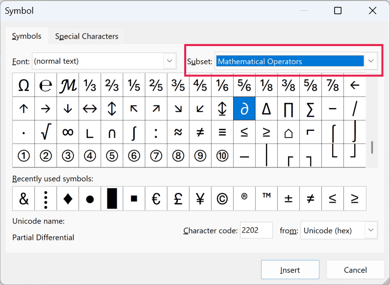
- In the Symbol dialog box, set the Subset drop-down to “Mathematical Operators.”
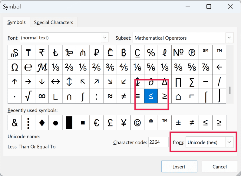
- Set the from box to Unicode (hex), select the ≤ symbol (character code 2264), click Insert, then click Close.
Once you’ve inserted it once, Excel keeps ≤ in the “Recently used symbols” strip at the bottom of the dialog, so it’s one click away next time.
Method #3: Using AutoCorrect
If you type the ≤ sign often, set up an AutoCorrect entry once and let Excel swap it in for you. You pick a short trigger, and Excel replaces it with ≤ as you type.
The steps below use Excel for Windows.
Here are the steps to create an AutoCorrect entry for the ≤ sign:
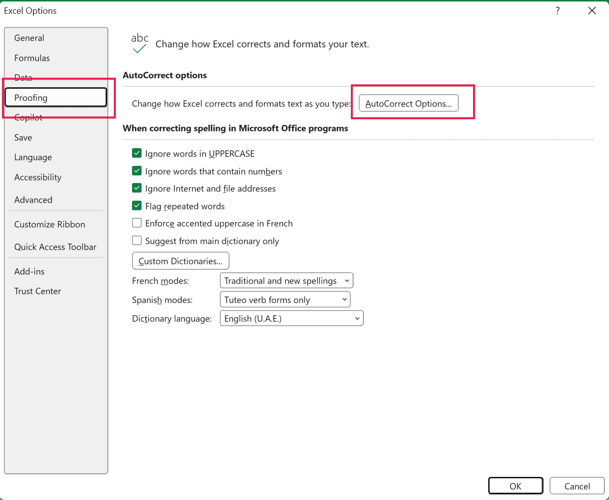
- Click File, then Options, then Proofing, then AutoCorrect Options.
- In the Replace box, type a short trigger such as ltoe. In the With box, paste or type the ≤ symbol.
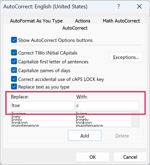
- Click Add, then click OK to close each dialog box.
With Replace text as you type enabled, typing ltoe and then pressing Space or Enter replaces it with ≤.
Note: Don’t use <= as your trigger text. That’s the comparison operator you type inside formulas, so an AutoCorrect entry on it can get in your way. Pick a trigger you’d never type otherwise, like ltoe.
Method #4: Using the UNICHAR Function
If you’d rather have Excel produce the symbol for you, UNICHAR builds it from the character’s Unicode number. The number for ≤ is 8804.
Here is the formula:
=UNICHAR(8804)
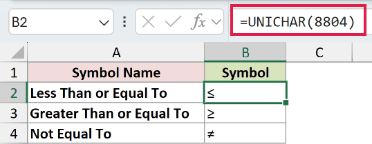
How does this formula work?
UNICHAR takes a Unicode code point and hands back the character it stands for. Feed it 8804 and you get ≤.
The same trick works for the two symbols either side of it. 8805 gives you ≥, and 8800 gives you ≠.
This one is handy when you are building a label inside a formula and need the symbol in the middle of the text.
Note: UNICHAR returns a formula result, not a typed character. If you need the plain symbol sitting in the cell, copy it and paste as values. CHAR(8804) won’t work here, because CHAR only handles codes 1 to 255. UNICHAR needs Excel 2013 or later.
Method #5: Copying and Pasting the Symbol
If you only need the ≤ sign once, the quickest route is to copy it from somewhere and paste it in. No codes, no dialog boxes.
Here is the symbol for you to copy:
≤
Select it, press Ctrl + C, click your cell in Excel, and press Ctrl + V.
If the pasted symbol brings formatting along with it, use Paste Special instead. Press Ctrl + Alt + V, choose Values, then click OK.
Additional Notes About the Less Than or Equal to Sign in Excel
- The ≤ symbol you insert as text is just a character. Excel treats it as text, so it won’t do any comparison. Write =IF(A1 ≤ 10,…) and Excel rejects the entry outright, because ≤ isn’t a valid operator. Use
<=when you need a real comparison. - The Symbol dialog box shows the character code as 2264. That’s the Unicode value in hex, which equals 8804 in decimal. 8804 is the number UNICHAR takes.
- Excel’s comparison operators are
=,<>,>,<,>=and<=. None of them has a single-glyph version, so ≤ will never work in place of<=inside a formula.
Frequently Asked Questions
What’s the difference between typing <= in a formula and inserting the ≤ symbol as text?
The <= operator tells Excel to compare two values and return TRUE or FALSE. The ≤ symbol is just a character for display. Excel never reads the glyph as an instruction to compare.
Why does my COUNTIF return 0 when the criteria cell shows ≤30?
Because ≤ is not an operator Excel understands. COUNTIF criteria have to read <=30 with the two characters. This usually happens when an AutoCorrect entry rewrote the cell behind your back, which is why Method #3 warns against using <= as a trigger.
How do I type the greater than or equal to sign (≥) in Excel?
Every method here works for ≥ too. Its Alt code is Alt + 242, its Unicode number is 8805 so =UNICHAR(8805) returns it, and it sits right next to ≤ in the Symbol dialog box.
Conclusion
Alt + 243 is the fastest way in once you know it, and the Symbol dialog box is the reliable option when you’d rather not memorize a code.
UNICHAR is the one to reach for when the symbol has to sit inside a formula, and copy and paste is fine for a one-off.
Pick whichever matches how often you need the sign, and you’ll never hunt for that missing key again.
Other Excel articles you may also like:
