UNICHAR Function in Excel

If you want to add a Unicode symbol from its decimal code, the UNICHAR function returns the matching character.

In this article, I’ll show you how to create symbols, label statuses, add product marks, and remove non-breaking spaces.

In Excel 2021 and later, you can feed UNICHAR a range and the results will spill into the cells below.

UNICHAR Function Syntax in Excel

The UNICHAR function uses the following syntax:

=UNICHAR(number)

• number is the decimal Unicode value for the character you want Excel to return.

When to Use UNICHAR Function

• Insert symbols in Excel when you know their decimal Unicode values.
• Create status marks from text labels or other conditions.
• Add registered or trade mark signs to names.
• Identify invisible Unicode characters when cleaning imported text.
• Generate several characters at once from a range of code points.

Example 1: Convert Unicode Codes to Symbols

Let’s start with a small Unicode reference list.

Below is a table of eight character names and their decimal Unicode codes.

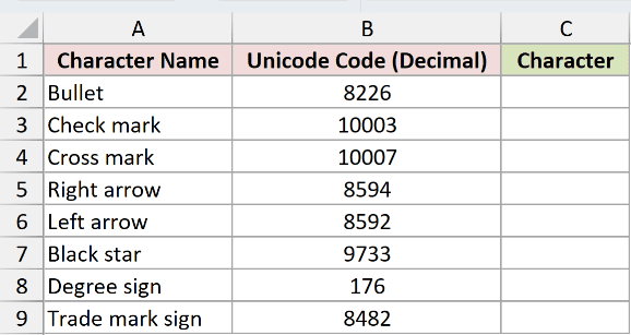
I want to convert every code in B2:B9 into its corresponding character.

Here is the formula:

=UNICHAR(B2:B9)

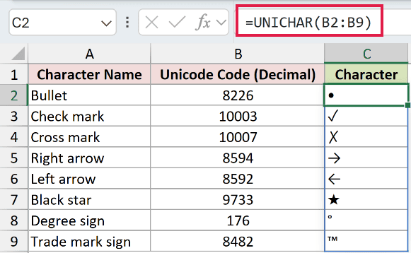
Because the formula receives a range, it returns eight characters and spills them down C2:C9.

The results are a bullet, check mark, cross mark, right arrow, left arrow, black star, degree sign, and trade mark sign.

For example, 8226 returns a bullet, 10003 returns a check mark, and 176 returns a degree sign.

Pro Tip: The character comes from the workbook’s font. If that font does not contain the requested glyph, Excel may show a box or another fallback symbol.

Example 2: Create Task Status Symbols

UNICHAR can sit inside a logical formula to return different symbols for different labels.

Below is a task list showing each owner and the status of their task.

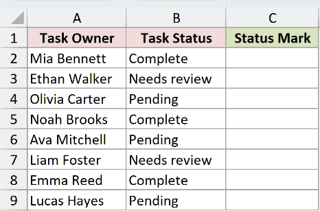
I want Complete to show a check mark, Needs review to show a cross mark, and Pending to show a bullet.

Here is the formula:

=IF(B2:B9="Complete",UNICHAR(10003),IF(B2:B9="Needs review",UNICHAR(10007),UNICHAR(8226)))

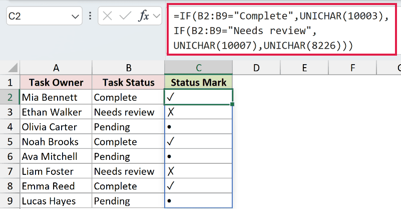
How this formula works:

• The IF function first checks whether each status equals Complete and returns the check mark from code 10003.
• The second IF checks for Needs review and returns the cross mark from code 10007.
• Every remaining status is Pending, so the formula returns the bullet from code 8226.

The spilled results are check mark, cross mark, bullet, check mark, bullet, cross mark, check mark, and bullet.

Example 3: Add Product Marks

You can join a UNICHAR result to existing text.

Below is a product list with either 8482 for a trade mark sign or 174 for a registered sign.

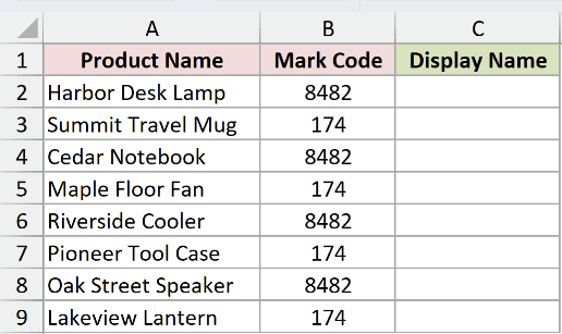
I want to append the symbol represented by each code to its product name.

Here is the formula:

=A2:A9&UNICHAR(B2:B9)

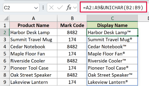
UNICHAR converts each code in B2:B9, and the ampersand joins that character to the matching product name.

The results alternate between names such as Harbor Desk Lamp™ and Summit Travel Mug® according to the code in each row.

Pro Tip: Add a normal space before UNICHAR if you want separation between the text and symbol. This example joins the marks directly to each name.

Example 4: Remove Non-Breaking Spaces

UNICHAR can also help you find invisible characters in imported text.

Below is a list of names containing non-breaking spaces at the beginning, end, or both. Those spaces often arrive with text copied from web pages.

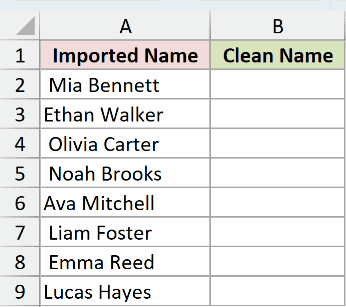
I want to replace the non-breaking spaces with normal spaces and remove the extra spacing around each name.

Here is the formula:

=TRIM(SUBSTITUTE(A2:A9,UNICHAR(160)," "))

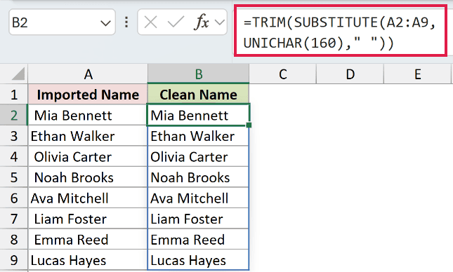
How this formula works:

• UNICHAR(160) returns the non-breaking space character.
• The SUBSTITUTE function replaces each non-breaking space with a regular space.
• The TRIM function removes the leading and trailing regular spaces from each name.

The formula spills eight cleaned names into B2:B9, from Mia Bennett through Lucas Hayes.

Tips & Common Mistakes

• UNICHAR is available in Excel 2016 and later. Range-based formulas spill in Excel 2021, Excel 2024, and Microsoft 365.
• In Excel 2019 and earlier, enter a single-cell formula such as =UNICHAR(B2) and fill it down.
• A zero or a numeric value outside the allowable Unicode range returns a #VALUE! error.
• Invalid partial surrogate values return a #N/A error.
• UNICODE does the reverse job. It returns the decimal code for the first character in a text string.
• The CHAR function returns a character from a code page, while UNICHAR uses a Unicode number. UNICHAR is the safer choice for Unicode symbols.
• Keep the expected output cells empty when using a range. A blocked result returns a #SPILL! error.

I covered how to generate Unicode characters, use them in labels, append marks, and clean non-breaking spaces.

I hope you found this article helpful.

List of All Excel Functions