
Excel’s INTERCEPT function returns the y-value where a best-fit straight line crosses the y-axis.
This is the fitted value when x is zero. Together with the slope, it lets you reconstruct the line from paired observations.
Treat it carefully when zero lies far outside the observed x-values. The fitted intercept may not represent a realistic starting value for that situation.
In this article, I’ll show you how to measure a zero-load offset, rebuild a fitted line, and calculate an intercept for filtered data.
INTERCEPT Function Syntax in Excel
INTERCEPT calculates the fitted value of y when x equals zero.
=INTERCEPT(known_y's,known_x's)
known_y'scontains the dependent values you want the fitted line to explain.known_x'scontains the corresponding independent values.
The y-values come first. Excel uses both ranges to fit a straight line, then returns its y-intercept.
When to Use the INTERCEPT Function
- Estimate a baseline value when the input or activity level is zero.
- Find a calibration offset from measured and reference values.
- Rebuild a fitted line with the INTERCEPT and SLOPE functions.
- Calculate a separate baseline for one group in a mixed dataset.
- Diagnose data that cannot produce one unique regression line.
Example 1: Check a Scale’s Zero-Load Offset
Let’s start with a small calibration example.
Below are five reference weights and their scale readings, plus an empty cell for the estimated reading at zero load.
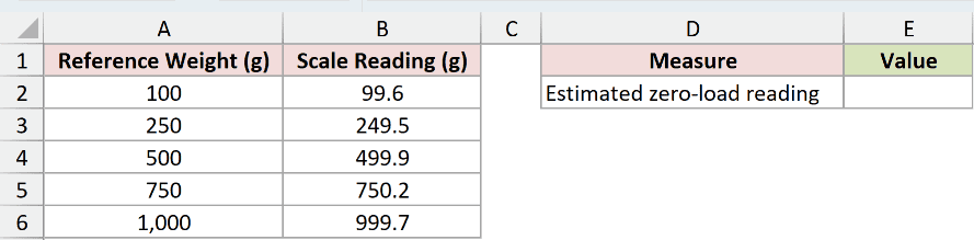
I want to estimate what the scale would read when the reference weight is zero.
Enter this formula in cell E2:
=INTERCEPT(B2:B6,A2:A6)
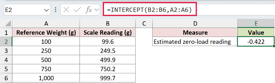
B2:B6 contains the scale readings, so it is the known_y's range. A2:A6 contains the reference weights and supplies known_x's.
The formula returns -0.422 grams. The fitted line suggests the scale would read slightly below zero with no weight on it.
Zero lies outside the measured x-values in this dataset. Treat the result as an extrapolated calibration estimate, not a direct measurement.
Example 2: Rebuild a Fitted Line
INTERCEPT and SLOPE can give you both parts of the fitted line y = mx + b.
Below are daily production levels and electricity use, with a calculation area for the baseline, slope, future production, and estimated use.
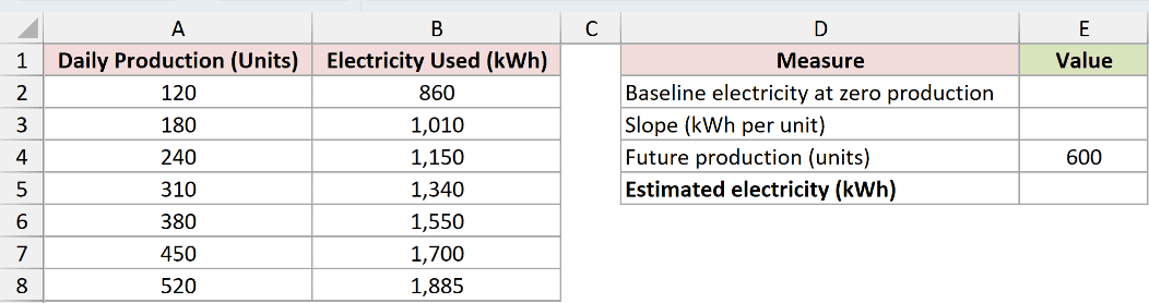
I want to estimate electricity use at 600 units by calculating the fitted baseline and slope first.
Enter this INTERCEPT formula in cell E2:
=INTERCEPT(B2:B8,A2:A8)
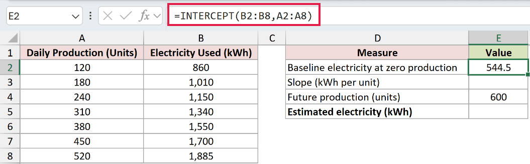
The result is 544.5 kWh. This is the fitted baseline electricity use when production is zero.
Enter this SLOPE formula in cell E3:
=SLOPE(B2:B8,A2:A8)
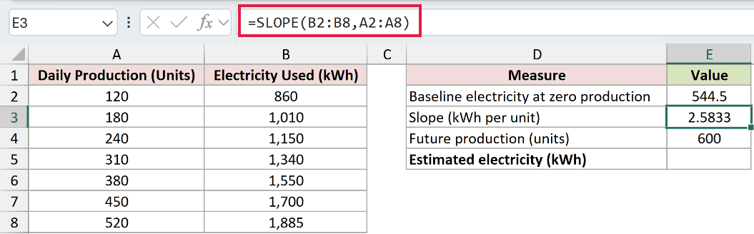
SLOPE returns 2.5833 kWh per unit. This is the fitted increase in electricity use for each additional production unit.
Cell E4 contains the future production level of 600 units. Enter this fitted-line formula in cell E5:
=E2+E3*E4
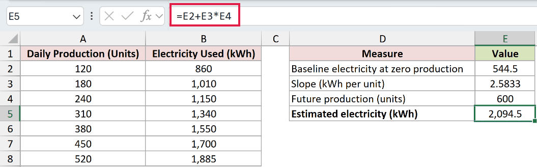
The formula adds the 544.5 baseline to the variable use for 600 units. It returns an estimated 2,094.5 kWh.
FORECAST.LINEAR can return the same type of prediction in one formula. INTERCEPT is useful when you also need the baseline as a separate result.
Example 3: Use INTERCEPT With FILTER
You can calculate a baseline for one group without copying that group’s rows to another range.
Below is a mixed table of online and in-store traffic with support-ticket counts. Cell E2 selects the online channel.
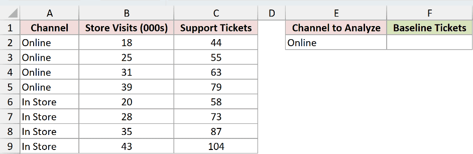
I want to calculate the fitted baseline tickets using only the online rows.
Enter this formula in cell F2:
=INTERCEPT(FILTER(C2:C9,A2:A9=E2),FILTER(B2:B9,A2:A9=E2))
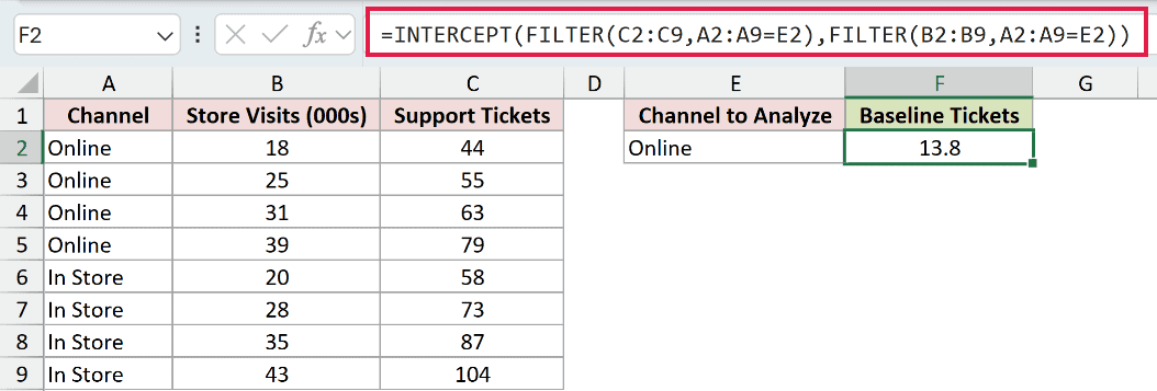
The first FILTER returns the online ticket counts for known_y's. The second returns the matching visit figures for known_x's.
INTERCEPT reduces those two filtered arrays to one value of 13.8 tickets. It does not spill a separate result for each row.
Pro Tip: FILTER is available in Excel 2021 and later. In Excel 2019 or 2016, copy each group to helper ranges or calculate the groups separately.
Example 4: Understand a Constant-X Error
INTERCEPT needs variation in the x-values to identify one best-fit line.
Below are five observations where every x-value is 1 and every y-value is 0, with empty result cells for INTERCEPT and LINEST.
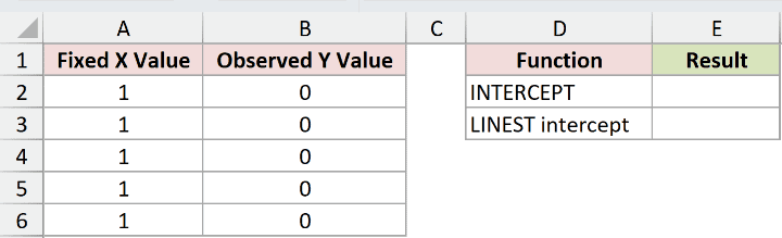
I want to compare how INTERCEPT and LINEST handle this undetermined, collinear dataset.
Enter this INTERCEPT formula in cell E2:
=INTERCEPT(B2:B6,A2:A6)
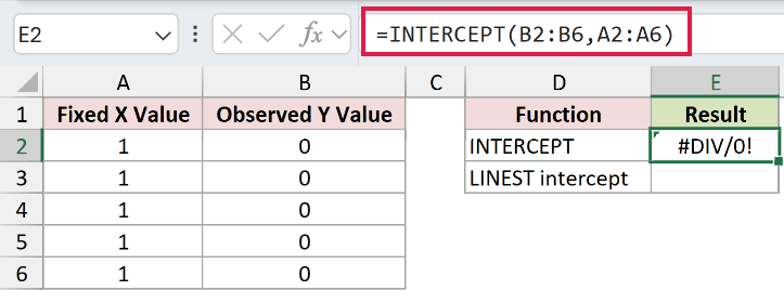
INTERCEPT returns #DIV/0!. With no variation in x, more than one line can satisfy the data, so the function cannot choose one intercept.
Enter this formula in cell E3 to extract the LINEST intercept:
=INDEX(LINEST(B2:B6,A2:A6),1,2)
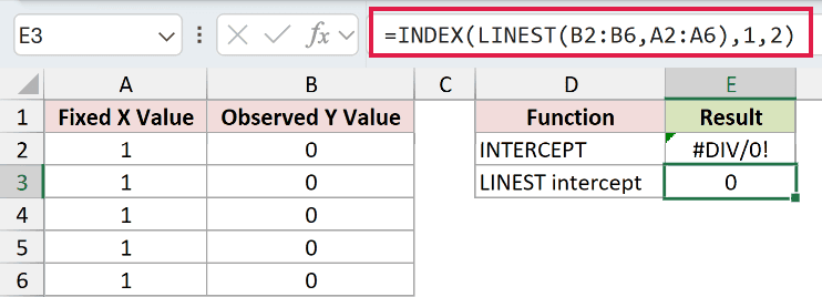
LINEST uses a different algorithm for collinear data and returns 0 here. That difference is documented by Microsoft.
Pro Tip: A LINEST result is not a repair for a constant-x INTERCEPT error. Check the source data and decide whether a regression line is meaningful.
Tips & Common Mistakes
- Put the y-values first and the x-values second. Reversing the ranges changes the regression and gives you a different intercept.
- Keep both ranges the same size and make sure each contains data. Empty or mismatched ranges return
#N/A. - Text, logical values, and blank cells in a referenced range are ignored. Cells containing zero are included.
- A constant x-range can return
#DIV/0!because Excel cannot determine one unique slope and intercept. - Interpret the intercept in context. If x equals zero far outside your observed data, the result is an extrapolation and may not be practical.
- INTERCEPT returns one number and does not spill. You can still pass it arrays created by FILTER in Excel 2021 and later.
- Use a scatter chart with a linear trendline when you want to see the fitted relationship and equation visually.
I have shown you how to use INTERCEPT for a baseline, combine it with SLOPE and FILTER, and diagnose a constant-x error.
I hope you found this article helpful.
Other Excel articles you may also like:
