If you want to fit a straight line to your data and pull out its slope, intercept, or full set of regression stats, the LINEST function does the math for you.
LINEST is a dynamic array function, so its results spill into a block of cells automatically.
In this article, I’ll show you how to use LINEST with practical examples, from a simple trend line to multiple regression.
LINEST Function Syntax in Excel
The LINEST function returns the statistics that describe a straight-line fit through your data.
=LINEST(known_ys, [known_xs], [const], [stats])
- known_ys – The known y-values, the thing you’re trying to predict or explain.
- [known_xs] – Optional. The known x-values, the predictors. Leave it out and Excel uses 1, 2, 3, and so on.
- [const] – Optional. TRUE (the default) calculates the intercept normally. FALSE forces it to zero.
- [stats] – Optional. TRUE returns the extra regression statistics. FALSE (the default) returns only the coefficients.
When to Use LINEST Function
- Find the slope and intercept of a trend in your data.
- Get R-squared, standard errors, and F-statistics for a regression.
- Run a multiple regression with several predictor columns.
- Pull regression coefficients straight into other formulas.
Example 1: Find the Slope and Intercept of a Trend
Let’s start with the most common use, a simple straight-line fit.
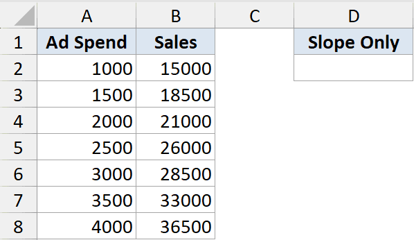
Below is the dataset with ad spend in column A and the sales it produced in column B.
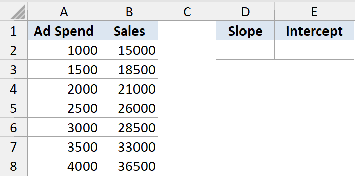
I want the slope and intercept of the line that best fits this relationship.
Here is the formula:
=LINEST(B2:B8,A2:A8)
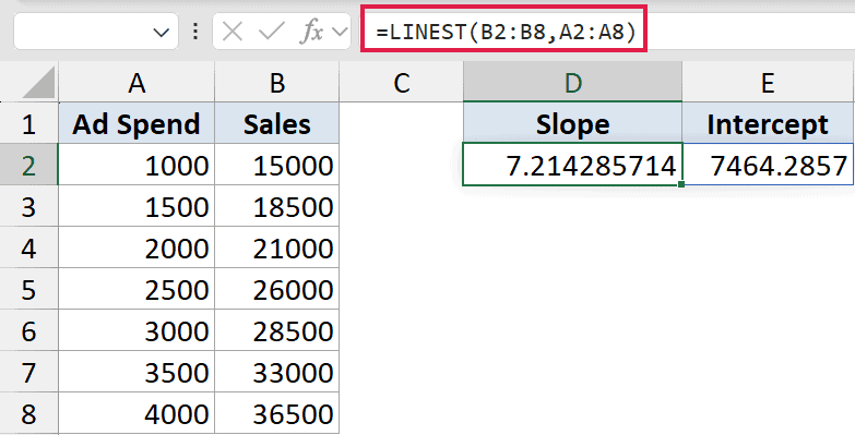
LINEST returns two numbers that spill across two cells. The first is the slope, about 7.21, and the second is the intercept.
The slope tells you sales rise by roughly 7.21 for every extra dollar of ad spend, and the intercept is where the line crosses zero.
Example 2: Get the Full Regression Statistics
Set the fourth argument to TRUE and LINEST hands you a full statistics block.
Below is the dataset with temperature in column A and ice cream sales in column B.
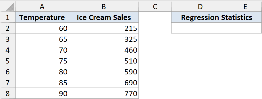
I want the slope and intercept plus the regression statistics that go with them.
Here is the formula:
=LINEST(B2:B8,A2:A8,TRUE,TRUE)
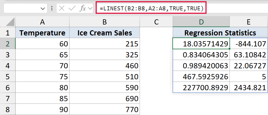
This spills a five-row block. Reading top to bottom, you get the coefficients, their standard errors, then R-squared with the standard error of the estimate, then the F-statistic with degrees of freedom, and finally the sums of squares.
The R-squared in the third row is the one most people look at. It tells you how much of the variation in sales the line explains.
Pro Tip: The statistics block always comes out in the same layout. Slope and intercept on top, then standard errors, R-squared, the F-test, and the sums of squares below. Keep a labeled copy nearby until you know it by heart.
Example 3: Run a Multiple Regression with Two Predictors
LINEST isn’t limited to one predictor. Give it several columns and it fits them all.
Below is the dataset with ad spend in column A, foot traffic in column B, and the resulting sales in column C.
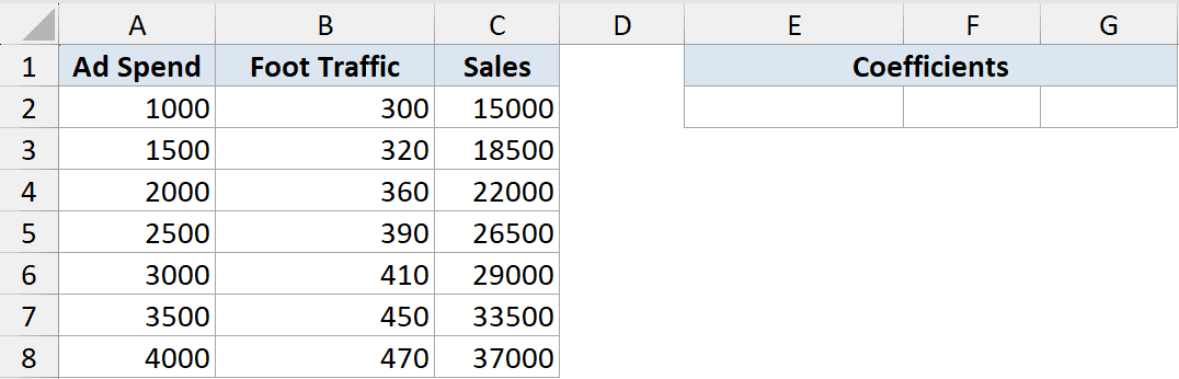
I want the coefficient for each predictor plus the intercept, all from one formula.
Here is the formula:
=LINEST(C2:C8,A2:B8)
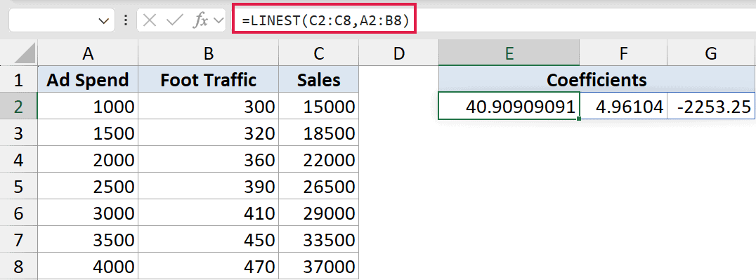
LINEST returns three values: a coefficient for each predictor and the intercept. There’s one catch that catches everyone out.
The coefficients come back in reverse order of your columns. So the first value is for foot traffic (the last predictor column), the second is for ad spend, and the last is the intercept.
Pro Tip: LINEST lists coefficients right to left compared to your predictor columns. Always read them in reverse, or you’ll match the wrong number to the wrong variable.
Example 4: Force the Line Through Zero
Sometimes the line should start at the origin, like when zero input must mean zero output.
Below is the dataset with hours studied in column A and the test score in column B.
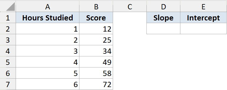
I want the slope of a line that’s forced to pass through zero, so no studying means a score of zero.
Here is the formula:
=LINEST(B2:B7,A2:A7,FALSE)
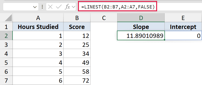
Setting the third argument to FALSE forces the intercept to zero. LINEST then finds the best slope under that constraint.
The intercept comes back as zero, and the slope adjusts to fit the line through the origin. Only use this when zero input genuinely should give zero output.
Example 5: Pull Out Just the Slope with INDEX
Often you don’t need the whole array, just one number from it.
Below is the dataset with ad spend in column A and sales in column B.
I want only the slope, dropped into a single cell so I can use it elsewhere.
Here is the formula:
=INDEX(LINEST(B2:B8,A2:A8),1,1)
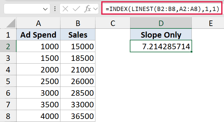
INDEX picks one value out of the LINEST array. The 1, 1 grabs the value in the first row and first column, which is the slope.
This is handy when you want to feed the slope straight into another calculation without the rest of the array spilling across your sheet.
Tips & Common Mistakes
- Coefficients come out in reverse. In multiple regression, LINEST lists the predictor coefficients right to left. Read them backward against your columns.
- Turn on stats with the fourth argument. Leave it out and you only get the coefficients. Set it to TRUE for R-squared, errors, and the F-test.
- Use INDEX to grab one value. When you need just the slope or intercept, wrap LINEST in INDEX rather than spilling the whole array.
- SLOPE and INTERCEPT are simpler for one line. If you only want the slope or intercept of a single predictor, the dedicated SLOPE and INTERCEPT functions are easier to read.
LINEST packs a full regression into one formula, and the dynamic array spill makes the output far easier to work with than the old method. Once you know the layout of the results and the reverse-order quirk, it’s a fast way to analyze trends right inside your sheet.
Try it on a trend of your own and pull out the slope, the stats, or the whole picture.
Related Excel Functions / Articles: