NA Function in Excel (4 Easy Examples)

If you want to mark a cell where no value is available, the NA function returns Excel’s #N/A error on purpose.

NA does not spill. It returns one #N/A error each time you call it.

In this article, I’ll show you how to flag missing calculation inputs, mark missing chart values, and distinguish blank inputs from unfound lookups.

Table of Contents

NA Function Syntax in Excel

The NA function takes no arguments and returns the #N/A error value.

=NA()

NA has no arguments, but the empty parentheses are required. Excel will not recognize it as a function if you leave them out.

You can type #N/A directly into a cell, but =NA() makes it clear that the error was added deliberately.

When to Use NA Function

Mark information that is currently unavailable instead of letting an empty cell be treated like zero.
Stop a dependent calculation when one of its required inputs is missing.
Pass an unavailable value to a chart source without substituting a misleading zero.
Distinguish a blank request from an unsuccessful lookup.

Example 1: Return the #N/A Error

We’ll start with the function on its own.

Below is the dataset with a status label in A1 and the cell where we want to show that no value is available in B1.

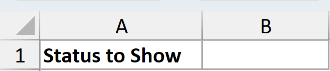
I want B1 to display the actual #N/A error value.

Here is the formula:

=NA()

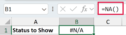
Excel displays #N/A in B1. This is an error value, not the text “N/A,” so formulas can recognize and handle it as an error.

Any formula that refers to B1 will normally return #N/A too. That propagation helps prevent calculations from quietly using incomplete data.

Pro Tip: You can type #N/A directly into a cell. I prefer =NA() because the formula bar makes the intention obvious.

Example 2: Flag Missing Calculation Inputs

Here’s a sales table where a calculation needs two inputs.

Below is the dataset with products, units sold, unit prices, and a Revenue column. Two rows are missing one required number.

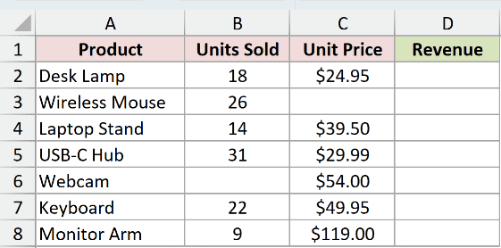
I want Revenue to show #N/A whenever Units Sold or Unit Price is blank, and calculate normally when both values are present.

Here is the formula in D2, filled down through D8:

=IF(OR(B2="",C2=""),NA(),B2*C2)

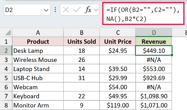
The OR function checks whether either input cell is blank. If one is blank, IF returns NA(); otherwise, it multiplies Units Sold by Unit Price.

D3 and D6 return #N/A because each row is missing an input. The completed rows return $449.10, $553.00, $929.69, $1,098.90, and $1,071.00.

This makes missing data visible and prevents a blank input from looking like a genuine zero-value sale.

Pro Tip: Use this pattern only when a missing input should stop the calculation. If a blank genuinely means zero, returning #N/A would misstate the data.

Example 3: Mark Missing Chart Values

This example prepares a clean source column for a chart.

Below is the dataset with eight weeks of registrations. Weeks 3 and 6 do not have actual values yet.

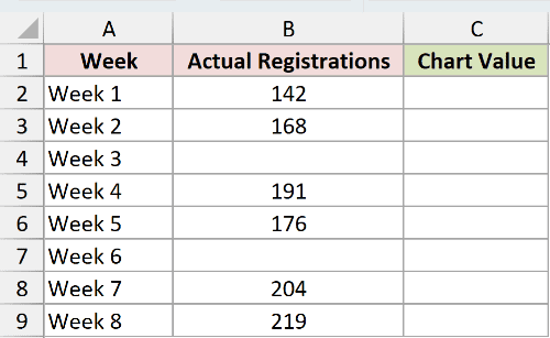
I want the Chart Value column to keep recorded registrations and return #N/A for weeks with no data.

Here is the formula in C2, filled down through C9:

=IF(B2="",NA(),B2)

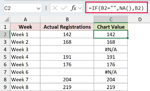
When Actual Registrations is blank, IF returns #N/A. Otherwise, the formula copies the recorded number into the chart source.

C4 and C7 show #N/A. The other rows preserve the values 142, 168, 191, 176, 204, and 219.

Unlike a zero, #N/A tells Excel that no numeric point is available. How a chart displays that point depends on its type, Excel version, and Hidden and Empty Cells settings.

Pro Tip: Check the finished chart instead of assuming every chart treats #N/A identically. Line, scatter, and radar charts offer settings that can change how unavailable points appear.

Example 4: Separate Blank and Unfound Lookups

Here’s a lookup where two kinds of missing result need different labels.

Below is an employee directory in columns A and B, plus submitted employee IDs and their lookup results in columns D and E.

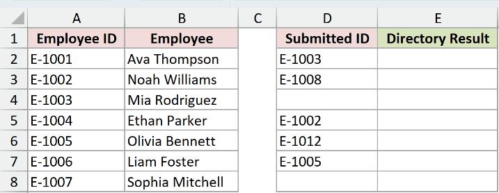
I want a blank submitted ID to return #N/A, while an ID that is entered but absent from the directory should return “Not found.”

Here is the formula in E2, filled down through E8:

=IF(D2="",NA(),XLOOKUP(D2,$A$2:$A$8,$B$2:$B$8,"Not found"))

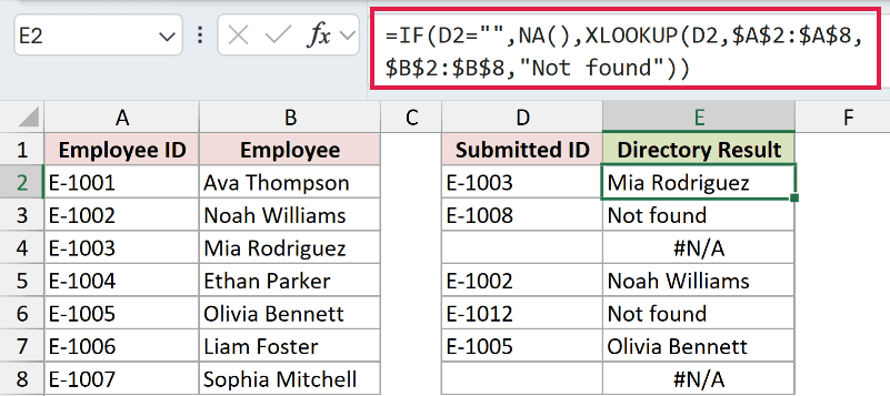
=IF(D2="",NA(),XLOOKUP(D2,$A$2:$A$8,$B$2:$B$8,"Not found")) in E2

IF checks the submitted ID first. A blank cell returns #N/A, which tells us no lookup was requested.

When an ID is present, XLOOKUP searches the directory. E-1003 returns Mia Rodriguez, while E-1008 and E-1012 return “Not found.”

The blank cells in D4 and D8 return #N/A. That keeps a missing submission separate from an ID that failed to match.

Pro Tip: XLOOKUP is unavailable in Excel 2016 and Excel 2019. In supported versions, its fourth argument handles the unmatched-ID message without hiding the separate NA() result for blanks.

Tips & Common Mistakes

Keep the empty parentheses. NA by itself is not a valid function call. Enter =NA() even though there are no arguments.
Do not confuse #N/A with text. The value returned by NA() is an Excel error. A typed string such as “N/A” is ordinary text and behaves differently in formulas.
Expect the error to propagate. A formula that refers to a cell containing #N/A normally returns #N/A too. Use IFNA only when you deliberately want to replace that error later.
Do not use #N/A as a permanent substitute for known data. Replace the error once the missing value becomes available.
Check chart settings. Chart type and Hidden and Empty Cells options can change how unavailable points appear, so verify the result in the chart you are using.
NA is scalar. It takes no range argument and returns one error value per call. Fill the formula down when several rows need separate #N/A results.

I use NA() when a blank should mean unavailable rather than zero. The examples above show how it marks missing inputs, prepares chart sources, and separates blank lookup requests.

I hope you found this article helpful.

List of All Excel Functions

Other Excel articles you may also like:

ISERR Function in Excel