
The ISERR function in Excel checks a value or calculation and returns TRUE for any error except #N/A. It returns FALSE for #N/A and values that are not errors.
A #N/A value can mean “not available yet” rather than “something is broken.” ISERR lets you keep those placeholders while flagging errors that need attention.
In this article, I’ll show you how to count broken rows, preserve #N/A placeholders, and label errors for follow-up.
ISERR Function Syntax in Excel
The ISERR function takes one argument:
=ISERR(value)
- value (required) is the value, cell reference, or calculation you want to test.
When to Use ISERR Function
- Flag calculation errors while leaving #N/A placeholders alone.
- Count rows containing errors such as #DIV/0! or #VALUE!.
- Show different messages for missing lookup values and broken calculations.
- Filter a dataset to return only records that need fixing.
Example 1: Flag and Count Broken Rows
An inventory report is a useful place to start because it contains both genuine errors and values that haven’t arrived yet.
Below is the dataset. It shows stock and average daily sales, with columns for days of stock and error flags, plus a labeled count cell.
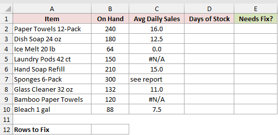
We want to calculate days of stock, flag the broken calculations, and count how many rows need fixing.
First, enter this formula in D2 and copy it down through D10:
=B2/C2
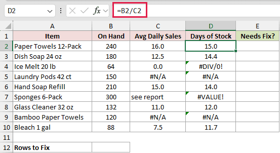
The division returns normal values for valid rows. Ice Melt returns #DIV/0!, while Sponges returns #VALUE! because its daily sales entry is text.
The #N/A results come from placeholders in the sales column. They mean the data hasn’t arrived yet, so we don’t want to treat them as broken rows.
Now enter this formula in E2:
=ISERR(D2:D10)
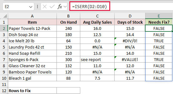
TRUE marks the #DIV/0! and #VALUE! rows, while the two #N/A rows stay FALSE. The results spill from E2 through E10.
Range-based ISERR formulas spill in Excel 2021, Excel 2024, and Microsoft 365. In Excel 2019 and earlier, test one cell and copy the formula down.
To count the TRUE results, use this formula in B12:
=SUMPRODUCT(--ISERR(D2:D10))
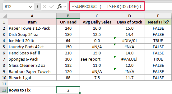
After the double unary converts the logical results to numbers, SUMPRODUCT returns 2.
ISERROR would count all four error rows because it includes #N/A.
Example 2: Keep Missing Months as #N/A
Here’s a monthly refund report where future months must remain unavailable rather than look like zero activity.
Below is the dataset. January through August contain real orders and refunds. September through December hold #N/A placeholders because that data hasn’t arrived.
The empty Refund Rate column will hold each monthly result.
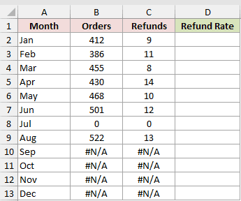
We want calculation errors to display as 0%, while the #N/A placeholders for months without data remain unchanged.
Enter this formula in D2:
=IF(ISERR(C2:C13/B2:B13),0,C2:C13/B2:B13)
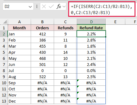
IF replaces only the calculations ISERR marks TRUE. Because ISERR returns FALSE for #N/A, the future-month placeholders continue to the output.
The shop was closed in July, so dividing 0 refunds by 0 orders produces #DIV/0!. ISERR catches it, and the displayed refund rate becomes 0.0%.
September through December contain #N/A placeholders because their data hasn’t arrived. ISERR returns FALSE for them, so the original #N/A results pass through.
Using IFERROR here would turn those future months into 0%. On a line chart, that would make the series drop to zero instead of stopping after August.
Pro Tip: Excel has no IFERR function. Use IF with ISERR when you need to replace calculation errors but preserve #N/A.
Example 3: Label Lookup and Input Errors
Now let’s separate missing job codes from labor-cost calculations with bad inputs.
Below is the dataset. It lists employees, job codes, hours, labor-cost and check columns, plus the hourly-rate table used by the lookup.
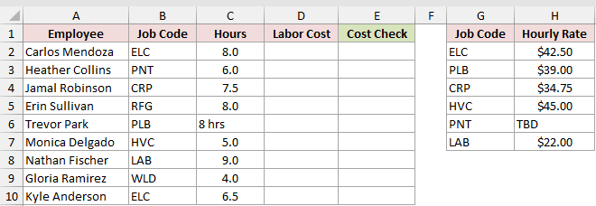
We want one message for a missing code and a different message when the hours or rate entry is invalid.
First, enter this labor-cost formula in D2 and copy it down through D10:
=C2*VLOOKUP(B2,$G$2:$H$7,2,FALSE)
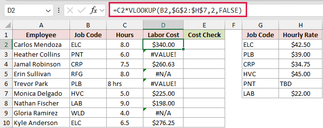
The formula multiplies each employee’s hours by the matching rate. Carlos Mendoza’s result is $340.00, and Jamal Robinson’s result is $260.63.
Heather Collins gets #VALUE! because the PNT rate is “TBD”. Trevor Park also gets #VALUE! because his hours are entered as “8 hrs”.
The RFG and WLD codes are missing from the rate table, so those lookups return #N/A as lookup errors.
Next, enter this formula in E2:
=IFNA(IF(ISERR(D2:D10),"Fix hours or rate",D2:D10),"Code not in table")
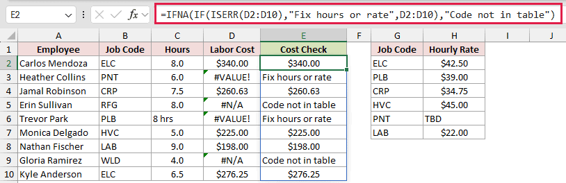
The inner ISERR test catches #VALUE! and lets valid labor costs pass through. The outer IFNA catches the #N/A results that ISERR deliberately leaves alone.
The final column displays “Fix hours or rate” for Heather and Trevor. It displays “Code not in table” for Erin Sullivan and Gloria Ramirez.
ISERR returns FALSE for a missing lookup because VLOOKUP returns #N/A. IFNA handles that error separately.
Example 4: Filter Records That Need Fixing
For the last example, we’ll turn an error test into a short exception list for a fleet manager.
Below is the dataset. It shows each driver’s miles and gallons, with a result area ready to list the logs that need fixing.
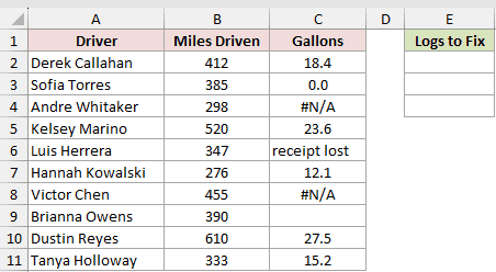
We want a list of drivers whose miles-per-gallon calculation produces an error other than #N/A.
Enter this formula in E2:
=FILTER(A2:A11,ISERR(B2:B11/C2:C11),"All logs OK")
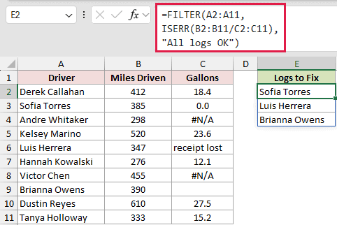
ISERR tests the miles divided by gallons expression without needing a helper column. FILTER then returns the driver names where that test is TRUE.
The spilled list contains Sofia Torres, Luis Herrera, and Brianna Owens. Sofia has zero gallons, Luis has text, and Brianna’s blank gallons cell counts as zero.
Andre Whitaker and Victor Chen have #N/A placeholders because their fuel-card data hasn’t synced. ISERR returns FALSE for those rows, so FILTER leaves them out.
FILTER and this range-based ISERR test require Excel 2021, Excel 2024, or Microsoft 365. In older versions, use an ISERR helper column and filter it for TRUE.
Tips & Common Mistakes
- ISERR returns TRUE for every Excel error except #N/A. That includes #DIV/0!, #VALUE!, #REF!, #NAME?, #NUM!, #NULL!, #SPILL!, and #CALC!.
- Don’t use ISERR alone to check whether MATCH found an item. A missing match returns #N/A, so ISERR returns FALSE. Use ISNA for that test.
- ISERROR catches every error, while IFNA and ISNA focus on #N/A.
Give #N/A its own handling path, and let ISERR drive the action for every other error.
Related Excel Functions / Articles:
