XLOOKUP Function in Excel Made Easy (with 7 Examples)

If you want to look up a value in one column and pull a matching value from another column, the XLOOKUP function is what you’re looking for.

It’s the modern replacement for VLOOKUP and HLOOKUP, and it fixes most of the things that used to trip people up.

In this article, I’ll show you how the XLOOKUP function works, with practical examples covering exact match, approximate match, looking to the left, returning multiple values at once, handling errors, and more.

One thing worth knowing up front. XLOOKUP plays really well with dynamic arrays in Excel 365. Pass it a single value, and you get one result. Pass it a range, or ask it to return multiple columns, and the output spills automatically into the surrounding cells. No fill-down, no Ctrl+Shift+Enter.

➡️ Click here to download the example file

Table of Contents

XLOOKUP Syntax

Here is the syntax of the XLOOKUP function:

=XLOOKUP(lookup_value, lookup_array, return_array, [if_not_found], [match_mode], [search_mode])

lookup_value – The value (or range of values) you want to look up. Pass a range here in Excel 365, and the result spills.
lookup_array – The range or array where you want to search for the lookup value.
return_array – The range or array from where you want the matching value returned. Can be a single column or row, or multiple columns/rows that spill the matching slice into adjacent cells.
[if_not_found] – Optional. The value to return when no match is found. If you skip this, XLOOKUP returns #N/A.
[match_mode] – Optional. Controls how the match is done. 0 (default) is exact match, -1 is exact match or next smaller, 1 is exact match or next larger, and 2 enables wildcards.
[search_mode] – Optional. Controls the search direction. 1 (default) searches first to last, -1 searches last to first, 2 is a binary search on an ascending list, and -2 is a binary search on a descending list.

When to Use XLOOKUP

Use this function when you need to:

Look up a value in a list and return a matching value from another column.
Look up many values at once and have the results spill into a column automatically.
Pull a value from a column that sits to the left of your lookup column.
Return an entire matching row (multiple columns) with a single formula.
Show a friendly message instead of #N/A when nothing matches.
Do an approximate match without sorting your data first.

Let me show you a few practical examples of how the XLOOKUP function works.

➡️ Click here to download the example file

Example 1: Look Up Many Values at Once

Let’s start with the most useful XLOOKUP pattern in Excel 365.

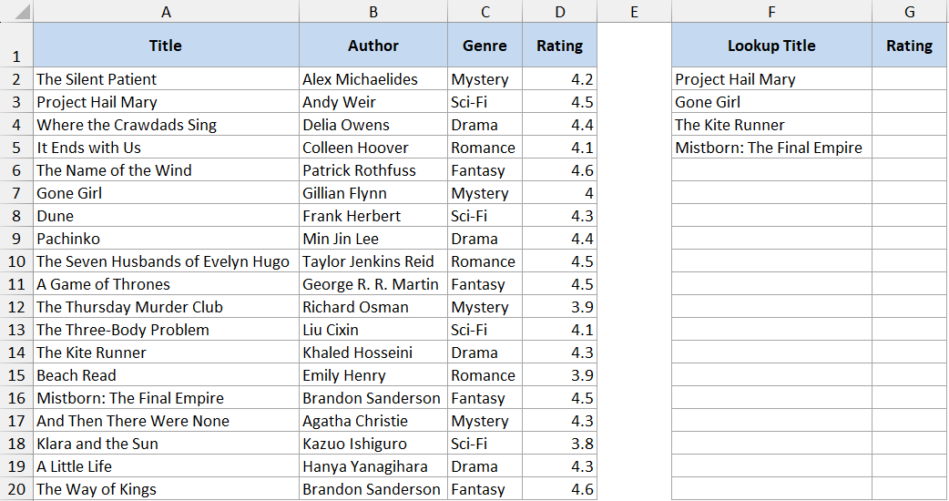
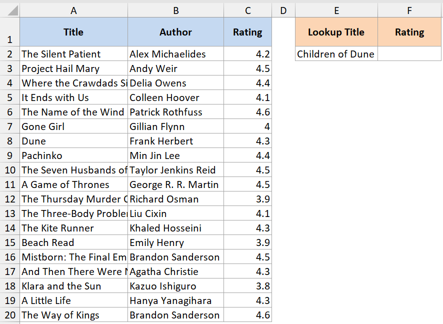
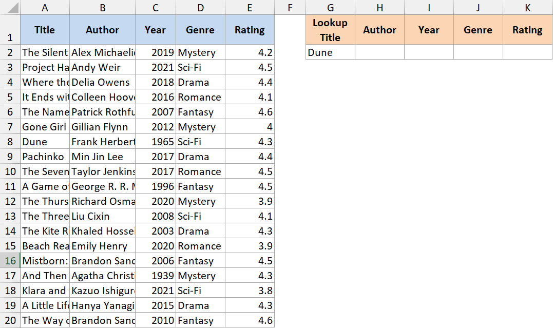
Below is a book catalog with the title, author, genre, and rating.

Separately, I have a short list of titles I want to grab the rating for. I want all the ratings to fill in with a single formula.

Excel dataset with book titles, authors, genres, and ratings alongside a lookup table for multiple XLOOKUP values

Here is the formula:

=XLOOKUP(F2:F5, A2:A20, D2:D20)

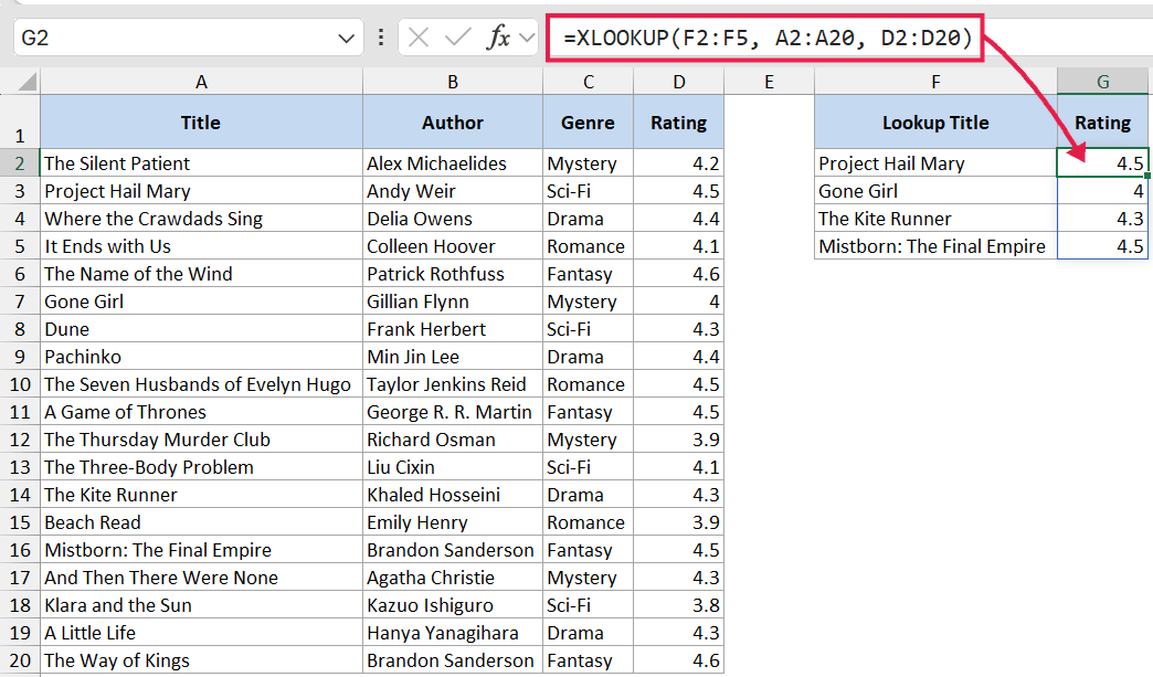
Excel XLOOKUP formula returning multiple values for a list of book titles and ratings in a table

In the above formula, F2:F5 is the column of titles I’m looking up.

A2:A20 is the full list of titles in the catalog, and D2:D20 is the rating column. Because lookup_value is a range, XLOOKUP returns four ratings and spills them right next to the lookup list.

You enter this formula once, in the top cell. The rest fills itself in. That’s the dynamic-array spill behavior. If you add or remove titles in the lookup list, the output adjusts on the spot.

By default, XLOOKUP does an exact match, so there’s no separate argument needed for that (although there is a match argument where you can specify approximate match, wild card, or exact match (or next smaller/greater value)).

This is already a nice change from VLOOKUP, where the default was an approximate match and caught a lot of people off guard.

Example 2: Look Up to the Left

Here’s something XLOOKUP does that VLOOKUP just cannot do.

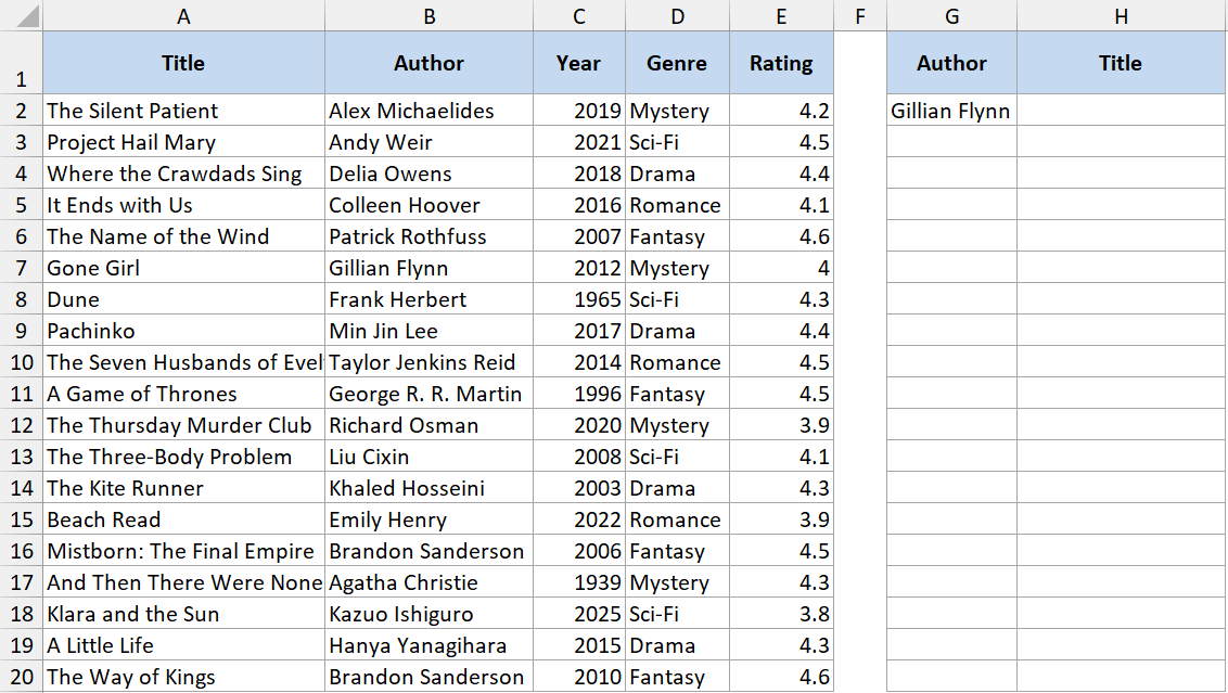
In the same catalog, the title sits in column A, and the author in column B. I want to find the title of the book when I have the name of the author.

Excel table showing XLOOKUP dataset used to look left from Author column G to retrieve Title in column H

Here is the formula:

=XLOOKUP(G2,B2:B20,A2:A20,"NA",0)

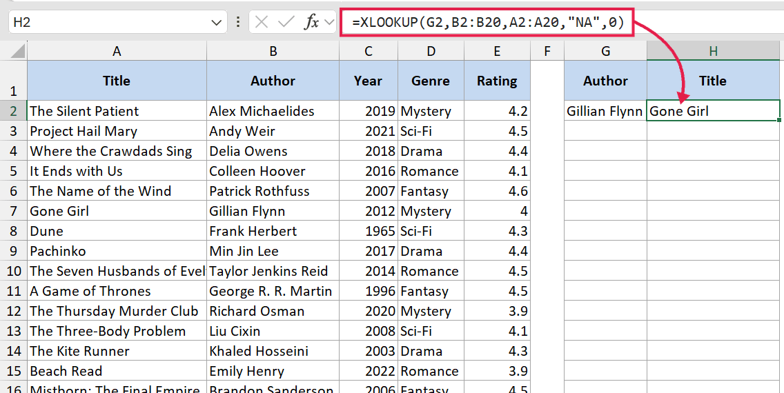
Excel formula bar showing XLOOKUP searching for an author in column B to return a book title from column A

What happens is XLOOKUP looks up the author name in B2:B20 and returns the matching title from A2:A20. The lookup column and return column don’t need to be in any particular order.

This is a common reason people switch from VLOOKUP to XLOOKUP. With VLOOKUP, you had to either rearrange your columns or fall back to an INDEX MATCH combination just to look to the left.

Example 3: Custom Message Instead of #N/A

This one is a small change that makes a big difference in real spreadsheets.

I’m searching for a title that may or may not be in the catalog. Instead of showing #N/A when there’s no match, I want it to say “Title not in catalog”.

Excel table showing an XLOOKUP formula returning a custom Not Found message for the book Children of Dune

Here is the formula:

=XLOOKUP(H2, A2:A20, E2:E20, "Title not in catalog")

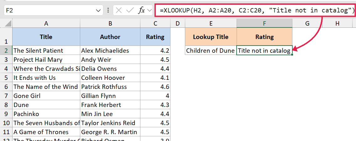
Excel XLOOKUP formula returning custom Title not in catalog text when a lookup value is not found in the source list

The fourth argument is the [if_not_found] value. If the title in H2 isn’t found, the formula returns “Title not in catalog” instead of #N/A.

This saves you from wrapping the whole thing in IFERROR, which is what people used to do with VLOOKUP. Cleaner formula, same result.

➡️ Click here to download the example file

Example 4: Approximate Match for Page-Length Tiers

Now let’s look at something more interesting.

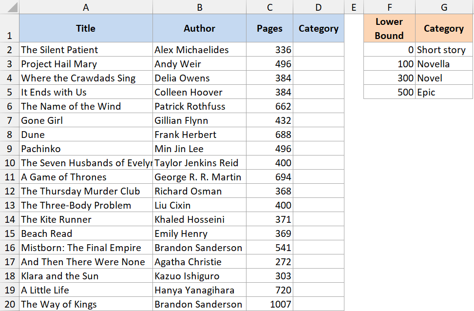
I have a small lookup table that classifies books by page count. Under 100 pages is a “Short story”, 100 to 299 is a “Novella”, 300 to 499 is a “Novel”, and 500+ is an “Epic”. I want to label every book in the catalog with the right category in one shot.

Excel dataset with book titles and page counts alongside a reference table for XLOOKUP range matching

Here is the formula:

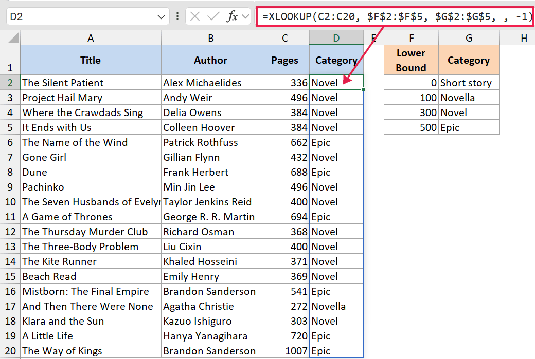
=XLOOKUP(C2:C20, $F$2:$F$5, $G$2:$G$5, , -1)

XLOOKUP formula bar showing approximate match with -1 mode to categorize book page counts based on a lower bound table

How this formula works:

C2:C20 is the page-count column for every book in the catalog.
$F$2:$F$5 is the lower bound of each tier (0, 100, 300, 500).
$G$2:$G$5 is the matching label.
The fourth argument is left blank, so any number outside the tier range returns #N/A.
The fifth argument, -1, tells XLOOKUP to find an exact match or the next smaller value.

Because lookup_value is a range, the result spills 19 categories into the cells below the formula. One formula, every row classified, no fill-down.

Unlike VLOOKUP’s approximate match, XLOOKUP doesn’t require the lookup list to be sorted. If you’re used to setting up tier lookups the old way, this is a good reason to compare it side by side with VLOOKUP approximate match.

Example 5: Return the Whole Matching Row at Once

This is one of my favorite XLOOKUP tricks.

I want to look up a book by title and return its author, year, genre, and rating, all at once with a single formula.

Excel dataset with book titles and attributes alongside a blank template for XLOOKUP to return a full row for Dune

Here is the formula:

=XLOOKUP(H2, A2:A20, B2:E20)

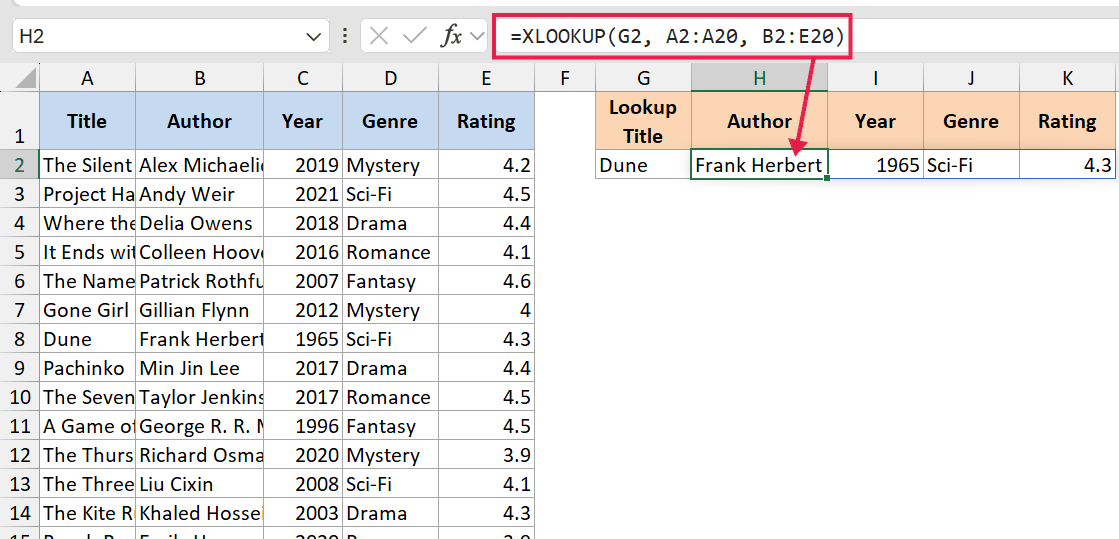
Excel formula bar showing XLOOKUP returning an entire row of book data into cells H2 through K2

Here, the return_array is B2:E20, which is four columns wide. XLOOKUP returns all four matching values and spills them across the cells to the right.

You enter the formula once. As long as the cells next to it are empty, the rest of the row fills itself in. This is one of the cleanest payoffs of the dynamic-array model in 365.

Example 6: Two-Way Lookup with Nested XLOOKUP

Let’s step it up with a more advanced use case.

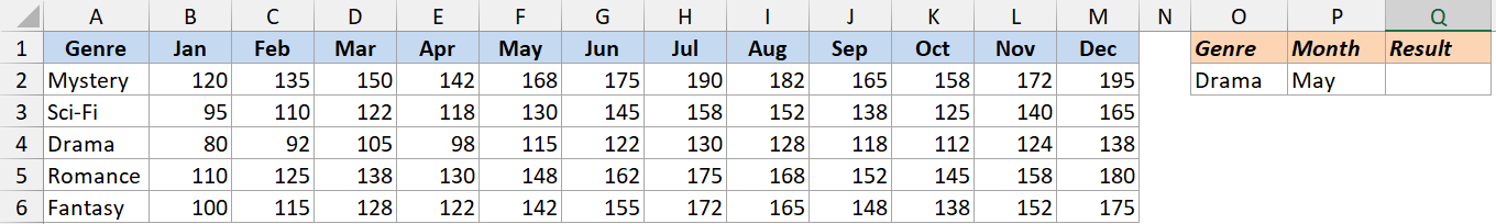
I have a checkout table that tracks how many times each book genre was borrowed in each month of the year.

Months are column headers, genres are row labels. I want to find the checkout count for a specific genre in a specific month.

Excel dataset with genres and months, plus a lookup table for Drama and May to perform a 2-way XLOOKUP

Here is the formula:

=XLOOKUP(O2, A2:A6, XLOOKUP(P2, B1:M1, B2:M6))

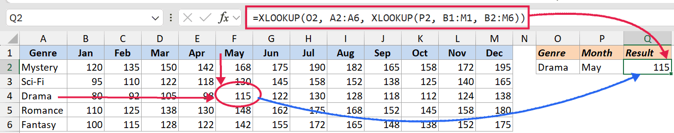
Excel formula bar showing a nested 2-way XLOOKUP function pointing to a specific cell value in a data table

How this formula works:

The inner XLOOKUP looks up the month (P2) in the column headers (B1:M1) and returns the matching column from the data (B2:M6).
The outer XLOOKUP then looks up the genre (O2) in the row labels (A2:A6) and returns the value from that single column.

This replaces the classic INDEX/MATCH/MATCH combination with two XLOOKUPs, which most people find easier to read.

Example 7: Multi-Criteria Lookup

This one comes up all the time when one column alone isn’t unique enough.

The library carries some titles in multiple formats (hardcover, paperback, ebook), so a title alone doesn’t uniquely identify a row. I want to look up the price for a specific title-and-format combination.

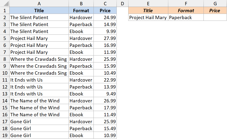
Excel table showing a multi-criteria XLOOKUP setup to find the price of a specific book title and format

Here is the formula:

=XLOOKUP(1,(A2:A19=E2)*(B2:B19=F2),C2:C19)

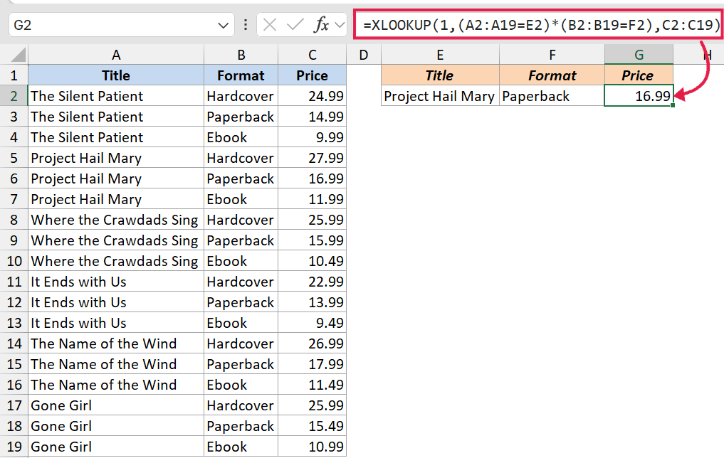
Excel formula bar showing XLOOKUP with multiple criteria to retrieve a price from a table based on title and format

How this formula works:

(A2:A19=E2) returns an array of TRUE/FALSE for each title match.
(B2:B19=F2) does the same for each format match.
Multiplying the two arrays gives 1 only where both are TRUE, and 0 otherwise.
XLOOKUP then looks for the value 1 in that combined array and returns the matching price from C2:C19.

If you have wildcard text patterns to deal with instead of exact criteria, take a look at wildcards in XLOOKUP for that approach.

Tips & Common Mistakes

#N/A errors: If you get #N/A, the lookup value isn’t in the lookup array. Check for extra spaces, different case, or numbers stored as text. Use the fourth argument to show a friendly message instead. The same kinds of issues that cause VLOOKUP not to work apply to XLOOKUP too.
#VALUE error from mismatched ranges: The lookup_array and return_array must be the same size (same number of rows for a vertical lookup, same number of columns for a horizontal one). If they’re not, XLOOKUP returns #VALUE.
#SPILL error: XLOOKUP spills whenever lookup_value is a range, return_array is multiple columns wide, or both. The cells the result needs to spill into must be empty. If something is in the way, you get #SPILL. Clear the spill range and the formula recalculates.
Reference the spilled output with the # operator: If your XLOOKUP lives in cell I2 and spills down a column, refer to the full spilled range as I2# in any downstream formula. The reference auto-resizes when the spill grows or shrinks, so charts and summaries built on I2# always track the live result.
Watch for the @ implicit intersection: Older Excel versions sometimes auto-insert an @ symbol when they save a workbook (e.g. =@XLOOKUP(...)). That collapses the spill to a single cell. Remove the @ and the spill comes back.
Compatibility: XLOOKUP is only available in Excel for Microsoft 365, Excel 2021, Excel for the web, and Excel for Mobile. If you share a file with someone on Excel 2019 or earlier, the formula will not work for them.
Default match is exact: Unlike VLOOKUP, XLOOKUP defaults to exact match. You don’t have to add a 0 or FALSE at the end like you used to.

That covers the XLOOKUP function and how to use it for everyday lookups, left lookups, tier lookups, multi-column returns, and the spill-many-lookups-at-once pattern that 365 unlocks.

Once you start using it, you’ll find it’s hard to go back to VLOOKUP for most tasks. Try it out on your own data and see how much shorter your formulas get.

List of All Excel Functions