
Excel’s STDEVA function estimates the standard deviation of a sample while treating TRUE as 1 and FALSE or text in referenced cells as 0.
That behavior helps when status words or logical flags are genuine data. It can mislead you when text is only a note, such as “Cancelled.”
The examples show when STDEVA should count text as zero, when STDEV.S should ignore it, and how computed arrays change the result.
STDEVA Function Syntax in Excel
STDEVA accepts one required value and up to 254 additional values, references, ranges, or arrays.
=STDEVA(value1, [value2], ...)
- value1 (required) is the first value, reference, range, or array from your sample.
- value2, … (optional) are additional values, references, ranges, or arrays from the same sample.
When to Use STDEVA Function
- Measure variation when text markers in a referenced range genuinely represent zero.
- Calculate sample variation directly from TRUE/FALSE flags, with TRUE counted as 1 and FALSE as 0.
- Compare STDEVA with STDEV.S when text might be a note rather than a measured value.
- Calculate variation for a filtered group while deliberately preserving text as zero.
Example 1: Count Downtime as Zero
Let’s start with a packing log where the word “Down” carries real meaning.
Below is the dataset. Column A lists work dates, column B records cases packed, and the labeled cell below will hold the daily output standard deviation.
Cell B6 for 7/3/2026 is blank because that day was a holiday.
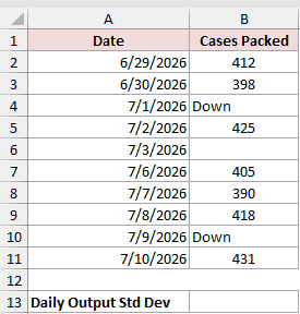
We want the sample standard deviation with each “Down” entry treated as zero and the blank holiday skipped.
Here is the formula:
=STDEVA(B2:B11)
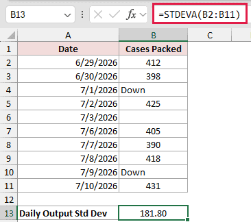
The formula returns 181.80. STDEVA counts each “Down” entry as 0 because it is text inside a reference.
The blank cell is different. STDEVA ignores it, so the holiday does not become another zero-output day.
STDEVA reduces the entire range to one result. It does not spill a result for each row.
Pro Tip: Use a text marker only when zero is what that marker truly means. Otherwise, STDEVA can make the variation look much larger than it is.
Example 2: Compare STDEVA and STDEV.S
A delivery log shows why treating text as zero can be the wrong choice.
Below is the dataset. Column A contains delivery IDs, column B holds delivery times and cancellation notes, and the labeled cells below will show both standard deviations.
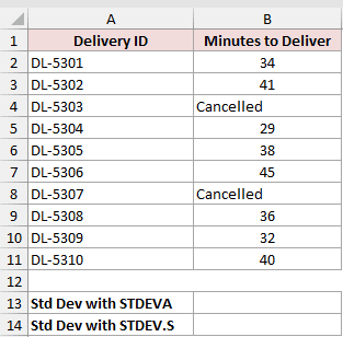
We want to see how STDEVA and STDEV.S handle the cancellation notes in the same range.
Here is the STDEVA formula:
=STDEVA(B2:B11)
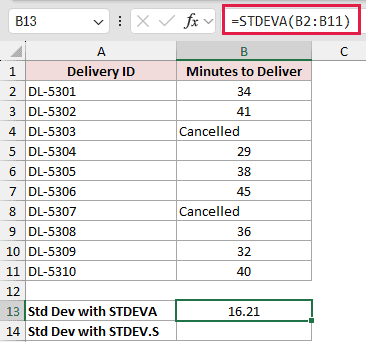
STDEVA returns 16.21 because every “Cancelled” entry becomes 0 in the calculation.
A cancelled delivery did not take zero minutes, so that interpretation is misleading. We need a function that ignores those notes instead.
Here is the STDEV.S formula:
=STDEV.S(B2:B11)
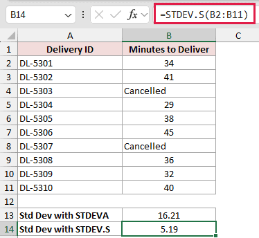
STDEV.S ignores the text and returns 5.19 from the recorded delivery times.
Use STDEVA when text means zero. Choose STDEV.S when text is only a note or status.
Example 3: Measure TRUE/FALSE Variation
Here’s a useful way to analyze quality checks stored as logical values.
Below is the dataset. Column A lists hourly checks, columns B and C contain each shift’s TRUE/FALSE results, and the bottom row will show both standard deviations.
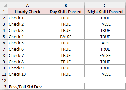
We want to measure how much each shift’s pass/fail results vary.
Here is the formula for the day shift:
=STDEVA(B2:B11)
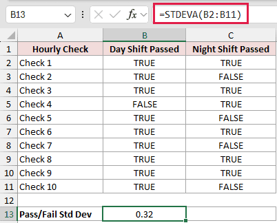
The day shift returns 0.32.
Here is the formula for the night shift:
=STDEVA(C2:C11)
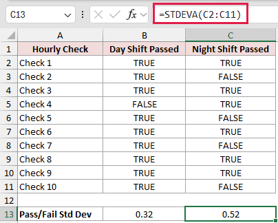
The night shift returns 0.52. STDEVA converts TRUE to 1 and FALSE to 0 before estimating the sample standard deviation.
The night shift’s 0.52 reflects a more mixed set of passes and failures. The day shift’s 0.32 comes from a column dominated by TRUE values.
Pro Tip: STDEV.S ignores logical values in a reference, so an all-TRUE/FALSE range returns #DIV/0!. STDEVA is the better fit when those flags are the data.
Example 4: Use STDEVA With FILTER
The last example calculates the variation in overtime hours for one department.
Below is the dataset. It lists employees, departments, and overtime hours. The first result cell is reserved for a deliberate FILTER-only mistake, and the second for the correction.
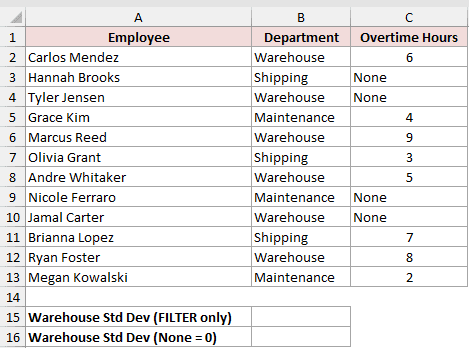
We want the Warehouse standard deviation while treating each “None” entry as zero overtime hours.
Here is the FILTER-only formula that demonstrates the mistake:
=STDEVA(FILTER(C2:C13,B2:B13="Warehouse"))
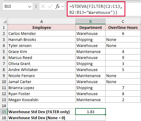
The white cell returns 1.83. This result demonstrates the FILTER-only mistake.
FILTER creates a computed array. In that array, STDEVA drops text and logical values, so the “None” entries disappear instead of becoming zeros.
We can preserve their meaning by converting text to 0 before FILTER passes the values to STDEVA.
Here is the corrected formula:
=STDEVA(FILTER(IF(ISTEXT(C2:C13),0,C2:C13),B2:B13="Warehouse"))
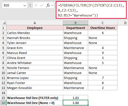
The corrected formula returns 3.88. IF changes text in the overtime column to 0, then FILTER keeps the Warehouse rows.
This distinction is easy to miss. Text in a worksheet reference counts as 0, but text passed through a computed array is ignored unless you convert it first.
Pro Tip: FILTER requires Excel 2021 or later. In Excel 2019 and earlier, copy the Warehouse rows to a separate range or sort them together, then point STDEVA at only those cells. Filtering alone only hides rows and does not change what STDEVA reads.
Tips & Common Mistakes
- STDEVA estimates standard deviation for a sample using the n-1 method. Use STDEVPA when your values represent the entire population.
- A number stored as text in a referenced cell counts as 0. Convert imported numeric text to real numbers before using STDEVA when zero is not intended.
- Non-numeric text typed directly as an argument returns #VALUE!. Text inside a worksheet reference follows the text-as-zero rule instead.
- Empty cells are ignored, but a formula returning an empty string is text and therefore counts as 0 inside a reference.
- Error values pass through STDEVA. Fix or filter the source error before calculating the standard deviation.
- STDEVA needs at least two counted entries. In a reference, these can be numbers, text, or TRUE/FALSE values. With fewer, it returns #DIV/0!.
- STDEVA always returns one result from its inputs. Dynamic array functions can prepare those inputs, but computed arrays change how text and logical values are handled.
STDEVA is useful when text and logicals carry real numeric meaning. If those entries are only notes, STDEV.S is usually the more honest choice.
Decide what zero means in your dataset before choosing between the two functions.
Other Excel articles you may also like:
