
Excel’s TOROW function converts a range or array into one horizontal row.
The function reads the source by row unless you choose column scanning. Its ignore setting can remove blank cells or errors from the returned row.
In this article, I’ll show you how to flatten grids, control scan order, and return open booking slots.
TOROW Function Syntax in Excel
The TOROW function accepts a source array and optional settings for ignored values and scan direction.
=TOROW(array, [ignore], [scan_by_column])
- array (required) is the range or array you want to reshape into one row.
- ignore (optional) uses
0to keep all values,1to ignore blanks,2to ignore errors, or3to ignore blanks and errors.0is the default when omitted, and blank cells return as 0. - scan_by_column (optional) tells TOROW to read down columns when TRUE. When FALSE or omitted, it reads across rows.
When to Use TOROW Function
- Flatten a rectangular data range into one horizontal list.
- Remove blank cells or errors while reshaping data.
- Change whether Excel reads a grid across rows or down columns.
- Turn a vertical list into a clean header row.
- Create a sorted list of distinct values collected from several columns.
Example 1: Flatten a Grid Into One Row
Let’s start with a warehouse pick grid.
Below is the dataset. Columns B through D hold warehouse codes for each aisle, and the Pick Route row shows where the spilled result will appear.
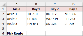
We want one horizontal pick route that follows the grid from left to right, then moves down to the next aisle.
Here is the formula:
=TOROW(B2:D4)
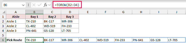
TOROW reads across the first source row, moves to the next row, and spills the codes horizontally from B6.
The route starts with TX-210, BK-117, and MR-306. It ends with PN-641, GS-128, and LT-705.
Example 2: Ignore Blank Cells With TOROW
Now let’s flatten a receipt grid without adding misleading zero amounts.
Below is the dataset. The weekday rows contain receipt amounts and blanks. The labeled rows beneath the grid hold the cleaned result and the default comparison.
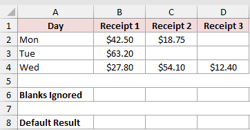
We want the horizontal list to contain only recorded receipt amounts.
Here is the formula:
=TOROW(B2:D4,1)
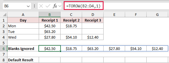
The ignore setting removes empty cells. The spilled row contains $42.50, $18.75, $63.20, $27.80, $54.10, and $12.40.
Here is the default formula for comparison:
=TOROW(B2:D4)
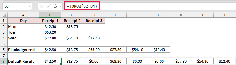
Without the ignore argument, blank source cells appear as $0.00 entries. The default row shows that comparison beside the cleaned receipt summary.
Pro Tip: Blank cells are not skipped by default. Use the ignore setting when a zero could be mistaken for a real transaction.
Example 3: Scan a Grid by Column
Here’s a rotation where each week should stay together.
Below is the dataset. Each week has a primary and backup person. The labeled rows beneath the schedule will hold the two scan-order results.
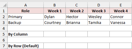
We want each primary person followed immediately by that week’s backup person.
Here is the column-scan formula:
=TOROW(B2:E3,,TRUE)
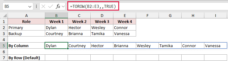
TRUE makes TOROW read down each week before moving right. The result begins Dylan, Courtney, Hector, Brianna and ends Wesley, Tamika, Connor, Vanessa.
Here is the default row-scan formula for comparison:
=TOROW(B2:E3)
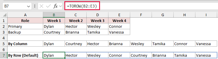
The default formula reads all primary names before all backup names. It returns Dylan, Hector, Wesley, Connor, Courtney, Brianna, Tamika, Vanessa.
The scan setting changes the order, not how many source values TOROW returns.
Example 4: Turn a Column Into a Header Row
TOROW also works when the source is a single column.
Below is the dataset. Column B lists course topics with empty weeks, and the Gradebook Header row provides space for the cleaned horizontal result.
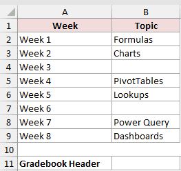
We want to turn the populated topics into a compact gradebook header.
Here is the formula:
=TOROW(B2:B9,1)
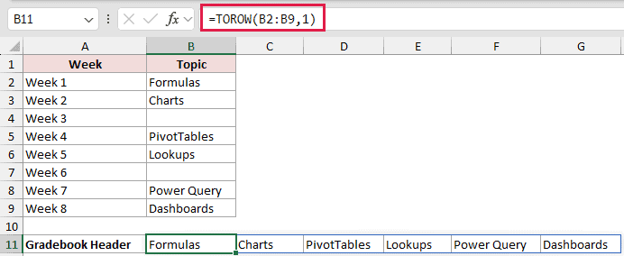
The formula skips the empty weeks and returns Formulas, Charts, PivotTables, Lookups, Power Query, and Dashboards across the row.
TRANSPOSE can also turn a column into a row. TOROW is handier here because it removes the blank topics in the same step.
Example 5: Create a Sorted Unique Row
Let’s combine TOROW with UNIQUE and SORT.
Below is the dataset. Each support ticket can have several tags, and the Unique Tags row is ready for the cleaned horizontal list.
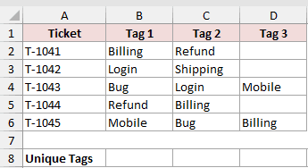
We want one alphabetical row containing each tag once.
Here is the formula:
=SORT(UNIQUE(TOROW(B2:D6,1),TRUE),,,TRUE)
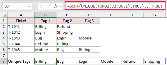
TOROW first flattens the tag grid and removes blanks. UNIQUE drops repeated tags, while SORT arranges the remaining values alphabetically.
The first TRUE tells UNIQUE to compare columns. The final TRUE tells SORT to sort columns because the list runs across a row.
The result is Billing, Bug, Login, Mobile, Refund, and Shipping.
You could also build a vertical unique list with TOCOL, then use TRANSPOSE. The TOROW version keeps the entire job horizontal.
Example 6: Return Open Booking Slots
Finally, let’s use the ignore setting as a filter.
Below is the dataset. Rows show times, columns show rooms, and filled cells contain meetings. The Open Slots row will hold the available room-time labels.
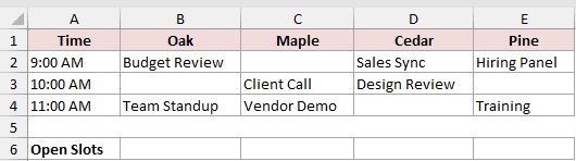
We want a horizontal list of every empty room and time combination.
Here is the formula:
=TOROW(IF(B2:E4="",B1:E1&" "&A2:A4,NA()),2)
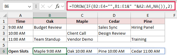
IF turns each empty booking cell into a room-time label. It returns #N/A for occupied cells, and TOROW removes those errors.
The available slots are Maple 9:00 AM, Oak 10:00 AM, Pine 10:00 AM, and Cedar 11:00 AM.
This pattern is useful when the condition must be checked across a rectangular grid rather than one list.
Tips & Common Mistakes
- TOROW is available in Microsoft 365 and Excel 2024 for Windows and Mac. Excel 2021 and earlier return #NAME?.
- Keep the cells to the right of the formula empty. Occupied cells block the spilled row and cause #SPILL!.
- Use a spill reference such as
B6#when another formula needs the complete TOROW result. - An array that is too large returns #NUM!.
We flattened grids, removed blanks, and changed the scan order.
We also combined TOROW with UNIQUE and SORT, then used IF and NA() to return open booking slots.
Related Excel Functions / Articles:
