
The WRAPCOLS function in Excel reshapes a one-dimensional list into a two-dimensional array, filling each column from top to bottom before starting the next column.
Its wrap_count argument sets the number of values per column. It does not set the number of columns, which is an easy detail to misread.
In this article, I’ll show you how to control padding, wrap a horizontal timeline, and calculate the column height for a requested layout.
WRAPCOLS Function Syntax in Excel
The WRAPCOLS function uses the following syntax:
=WRAPCOLS(vector, wrap_count, [pad_with])
- vector (required) is the single row or single column you want to reshape.
- wrap_count (required) is the maximum number of values placed in each output column.
- pad_with (optional) is the value used to fill unused cells in the final column. Excel uses #N/A when you omit it.
When to Use WRAPCOLS Function
- Turn a long vertical list into a shorter layout that is easier to print or scan.
- Split a horizontal timeline into one column for each reporting period.
- Arrange sorted names or items into a compact directory.
- Combine separate lists before placing them into a column-based layout.
- Remove blank entries before wrapping a list.
Example 1: Wrap a List Into Columns
Let’s start with the basic WRAPCOLS pattern.
Below is the dataset. Column A contains the new-hire list, while columns C through E provide the empty result area with matching headers.
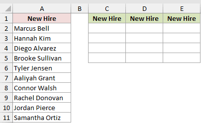
We want to arrange the names with four values in each output column.
Here is the formula:
=WRAPCOLS(A2:A11,4)
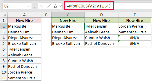
WRAPCOLS reads down A2:A11. It places Marcus Bell through Brooke Sullivan in the first column, then continues with Tyler Jensen at the top of the next column.
The last column contains Jordan Pierce and Samantha Ortiz. Its two unused cells display #N/A because the optional padding argument was omitted.
This is a native dynamic-array formula. Enter it once, and Excel spills the complete result across the empty output area.
Pro Tip: WRAPCOLS fills down each column first. WRAPROWS fills across each row first, so choose the function that matches how you want the result read.
Example 2: Replace Default Padding
Here’s a practical way to make unused cells meaningful.
Below is the dataset. Column A lists banquet guests, while columns C through E show the labeled seating area waiting for the wrapped result.
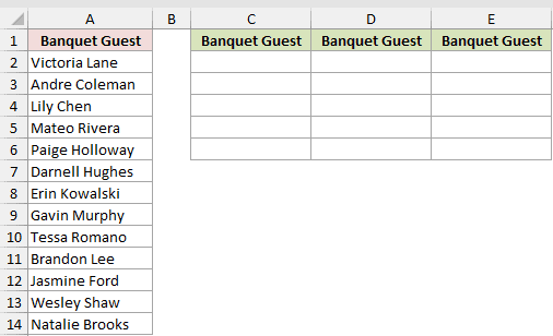
We want each column to hold five guests and mark any unused seat as Open.
Here is the formula:
=WRAPCOLS(A2:A14,5,"Open")
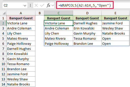
The third argument replaces the default #N/A padding. The Open entries in E5 and E6 mark the unused seats.
You can also use "" for padding when you want those unused cells to look blank.
Example 3: Wrap a Horizontal Timeline
WRAPCOLS also accepts a single horizontal row.
Below is the dataset. Row 2 contains quarterly revenue, and the lower table provides quarter labels with empty columns for the annual results.
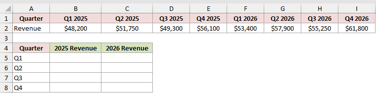
We want to turn the timeline into separate 2025 and 2026 revenue columns.
Here is the formula:
=WRAPCOLS(B2:I2,4)
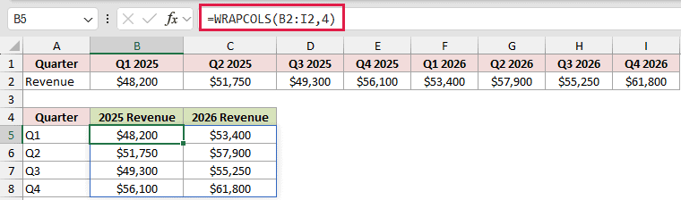
Excel takes the first four values for the 2025 column, from $48,200 through $56,100. It places the remaining values in the 2026 column.
That second column runs from $53,400 through $61,800, while the quarter labels in column A make the reshaped figures easy to compare.
Example 4: Target a Column Count
Now let’s calculate the column height instead of typing it directly.
Below is the dataset. Column A lists supply items, D1 holds the requested column count, C3:E3 contains the headers, and C4:E8 is the empty result area.
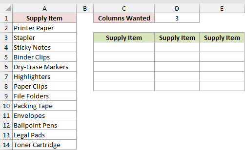
We want the list arranged across no more than the number of columns requested in D1.
Here is the formula:
=WRAPCOLS(A2:A14,ROUNDUP(ROWS(A2:A14)/D1,0),"")
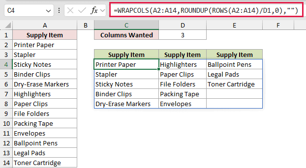
ROWS counts the source items. Dividing by D1 estimates the required column height.
ROUNDUP rounds that height up so the result stays within the D1 column count. Otherwise, WRAPCOLS truncates the height and adds another column.
WRAPCOLS then uses that height. The first output row contains Printer Paper, Highlighters, and Ballpoint Pens.
The result uses at most the number of columns requested in D1. Depending on how the item count divides, the result may use fewer columns.
The empty text padding keeps unused cells at the bottom of the final column visually blank.
Example 5: Sort Before Wrapping
Here’s how to build a compact directory that reads in alphabetical order.
Below is the dataset. Column A contains an unsorted vendor list, while columns C through E provide the empty directory layout.
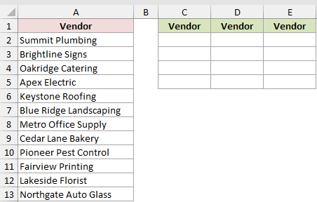
We want to sort the vendors before arranging them down the output columns.
Here is the formula:
=WRAPCOLS(SORT(A2:A13),4)
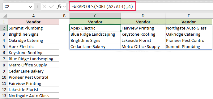
SORT creates the alphabetical vector first. WRAPCOLS then reshapes that sorted result without changing its order.
The directory begins with Apex Electric in C2, continues down the first column, and ends with Summit Plumbing in E5.
Reading down each column and then moving right keeps the complete list in alphabetical order.
Example 6: Combine Lists Before Wrapping
Sometimes the source values sit in separate columns.
Below is the dataset. Columns A and B hold online and walk-in signups, while columns D and E provide the empty attendee layout.
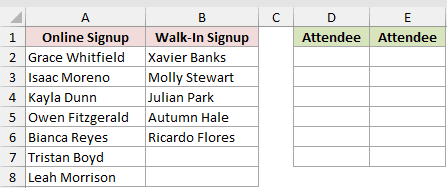
We want to combine both signup lists into one vector before wrapping the attendees.
Here is the formula:
=WRAPCOLS(VSTACK(A2:A8,B2:B6),6)
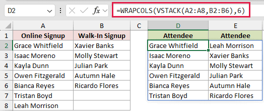
VSTACK places the online list above the walk-in list, creating the one-dimensional vector WRAPCOLS needs.
The wrapped result starts with Grace Whitfield in D2. The second output column begins with Leah Morrison and ends with Ricardo Flores.
Passing the two-column source directly to WRAPCOLS would return #VALUE! because WRAPCOLS requires a single row or single column.
Example 7: Skip Blank Source Cells
Blank cells need a little care because WRAPCOLS does not automatically ignore them.
Below is the dataset. Columns A and B list potluck guests and dishes, including blank dish cells, while columns D through F provide the empty result grid.
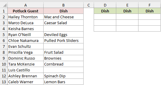
We want to remove the blank dishes before arranging the remaining entries into columns.
Here is the formula:
=WRAPCOLS(TOCOL(B2:B13,1),3)
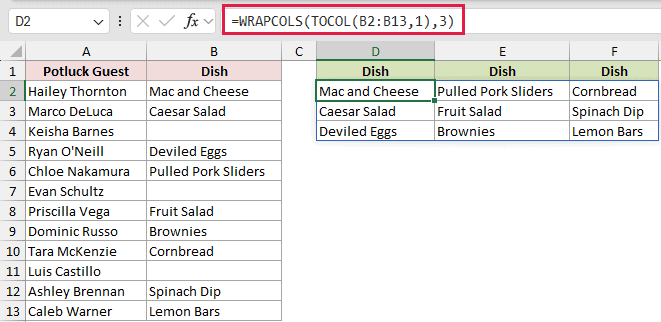
TOCOL prepares the source vector and ignores blank cells. WRAPCOLS then places three dishes in each output column.
The first column runs from Mac and Cheese through Deviled Eggs. The last column contains Cornbread, Spinach Dip, and Lemon Bars.
If you pass B2:B13 directly, each blank source cell appears as 0 and still takes a position in the wrapped result.
Tips & Common Mistakes
- WRAPCOLS is available in Microsoft 365 and Excel 2024. Excel 2021 and earlier return #NAME? because the function is unavailable there.
wrap_countmeans values per column, not the number of output columns.- Excel truncates a decimal
wrap_count. In testing, 2.7 behaved like 2. - A
wrap_countbelow 1 returns #NUM!, while a two-dimensional source returns #VALUE!. - Keep the spill area empty. A blocked destination causes #SPILL!, and spilled formulas cannot expand inside an Excel Table.
- Use the spill reference from the formula’s anchor when another calculation needs the complete wrapped result. For Example 1, that’s
C2#. - Omitting
pad_withproduces #N/A in unused cells. Supply an empty text value when you want blank-looking padding. - A blank source cell becomes 0. Clean the vector first when blanks should be excluded.
We used wrap_count to set values per column and replaced the default padding.
We also wrapped a horizontal row and calculated a column height from the requested column count.
The final examples prepared each source vector before WRAPCOLS reshaped it.
Related Excel Functions / Articles:
