
Excel’s COVARIANCE.S function returns the sample covariance between two sets of paired numeric observations.
The sign shows whether the pairs tend to move together or in opposite directions. The size depends on the units used, so it doesn’t show relationship strength by itself.
In this article, I’ll show you how to read the sign, compare sample and population covariance, and handle incomplete pairs.
COVARIANCE.S Function Syntax in Excel
The function takes two equally sized arrays or cell ranges containing paired observations.
=COVARIANCE.S(array1, array2)
- array1 (required) is the first range or array of numeric observations.
- array2 (required) is the second range or array paired row by row with the first.
When to Use COVARIANCE.S Function
- Check whether two measures in a sample tend to rise and fall together.
- Compare returns from two investments when reviewing how they move relative to each other.
- Measure covariance from a sample rather than an entire population.
- Verify a manual sample-covariance calculation that divides by
n - 1. - Calculate covariance for one group by passing filtered arrays to the function.
Example 1: Calculate Positive Sample Covariance
Let’s start with a straightforward sales example.
Below is the dataset. Column A lists the reps, columns B and C contain sales calls and closed deals, and E2 is reserved for sample covariance.
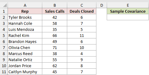
We want to measure how sales calls and closed deals vary together across this sample.
Here is the formula:
=COVARIANCE.S(B2:B11,C2:C11)
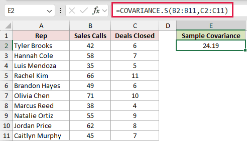
Excel returns 24.19. The positive sign indicates that reps with more calls generally closed more deals in this sample.
COVARIANCE.S reduces both paired ranges to one result and doesn’t return a separate covariance for each rep.
That single value describes how the observations move together, but it doesn’t prove that additional calls alone caused the extra deals.
Example 2: Interpret Negative Covariance
Now let’s look at two monthly return series that tend to move in opposite directions.
Below is the dataset. Column A lists the months, columns B and C contain fund returns, and E2 is the sample covariance answer cell.
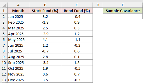
We want to measure how the stock and bond fund returns moved together during the period shown.
Here is the formula:
=COVARIANCE.S(B2:B13,C2:C13)
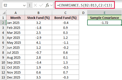
Excel returns -1.72 in percent-squared units. The negative sign means above-average returns in one series tended to accompany below-average returns in the other.
That doesn’t mean the funds moved opposite each other in every month. Covariance summarizes the overall paired movement across the sample.
Don’t compare its absolute size with covariance measured in different units. Use CORREL when you need a scale-free measure of relationship strength.
Example 3: Compare Sample and Population Covariance
Here’s where the difference between COVARIANCE.S and COVARIANCE.P becomes clear.
Below is the dataset. Columns B and C hold staff and revenue figures, while the labeled cells in columns E and F hold three covariance calculations.
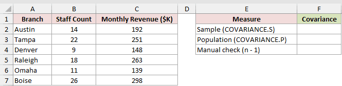
We want to compare the sample result, population result, and a manual sample-covariance check.
First, here is the sample formula:
=COVARIANCE.S(B2:B7,C2:C7)
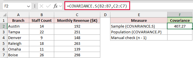
The sample covariance is 407.27.
Here is the population formula:
=COVARIANCE.P(B2:B7,C2:C7)
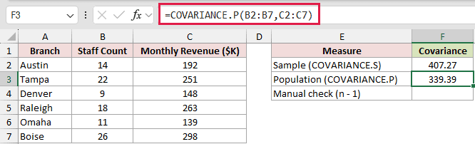
The population covariance is 339.39. COVARIANCE.P divides by n, while COVARIANCE.S divides by n - 1.
Finally, here is the manual sample-covariance check:
=SUMPRODUCT((B2:B7-AVERAGE(B2:B7))*(C2:C7-AVERAGE(C2:C7)))/(COUNT(B2:B7)-1)
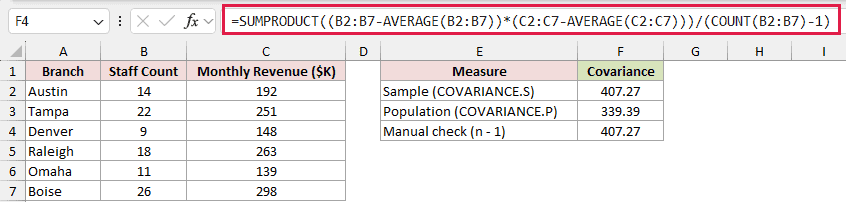
The manual calculation returns 407.27, matching COVARIANCE.S.
Use COVARIANCE.S when the rows represent a sample. Use COVARIANCE.P when the rows are the complete population you want to describe.
Example 4: Normalize Covariance With CORREL
This example shows why covariance size can be misleading.
Below is the dataset. Columns B and C contain square footage and sale price, while columns E and F provide labeled cells for three relationship measures.
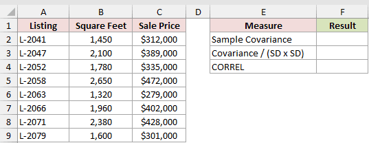
We want to calculate covariance, normalize it with both sample standard deviations, and confirm the normalized result with CORREL.
Here is the sample covariance formula:
=COVARIANCE.S(B2:B9,C2:C9)
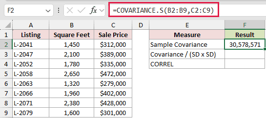
Excel returns 30,578,571. That looks large, but the value reflects the units used for square feet and sale price.
Here is the formula that divides covariance by both sample standard deviations:
=COVARIANCE.S(B2:B9,C2:C9)/(STDEV.S(B2:B9)*STDEV.S(C2:C9))
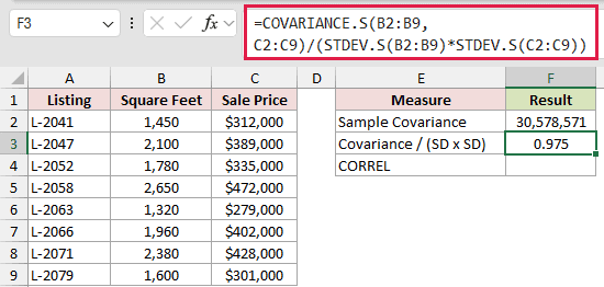
The normalized result is 0.975.
Here is the direct CORREL formula:
=CORREL(B2:B9,C2:C9)
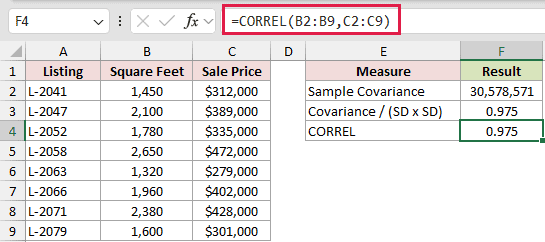
CORREL also returns 0.975. It expresses the same relationship without carrying the original measurement units.
Changing the units would change the covariance value, even though the underlying relationship remains the same. A large covariance doesn’t automatically mean a strong relationship.
Pro Tip: For the same ranges, dividing sample covariance by both sample standard deviations should match CORREL.
Example 5: Handle Text, Blanks, and Zeros
Real worksheets rarely contain perfectly complete numeric pairs.
Below is the dataset. Columns B and C contain displays and weekly units, including text, a blank, and a zero. Cell E2 will hold sample covariance.
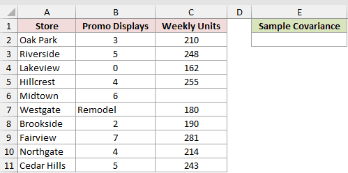
We want to see how COVARIANCE.S handles these mixed rows without cleaning the source first.
Here is the formula:
=COVARIANCE.S(B2:B11,C2:C11)
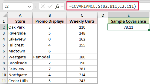
Excel returns 78.11 from the complete numeric pairs.
Midtown’s blank in C6 drops that row’s whole pair. Westgate’s weekly-units value in C7 is excluded along with the text in B7.
Lakeview’s zero in B4 stays in the calculation because zero is numeric data, not a blank.
Removing values independently would shift the remaining observations out of alignment and change what the rows mean.
Example 6: Calculate Covariance for Filtered Rows
Finally, let’s calculate covariance for one hub without creating helper columns.
Below is the dataset. Columns A to C contain hub activity, E2 stores the selected hub, and F2 is reserved for its sample covariance.
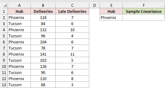
We want to calculate covariance only for the Phoenix rows selected in E2.
Here is the formula:
=COVARIANCE.S(FILTER(B2:B13,A2:A13=E2),FILTER(C2:C13,A2:A13=E2))
FILTER needs Excel 2021, Excel 2024, or Microsoft 365.
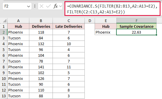
Excel returns 22.63 for Phoenix.
Each FILTER call keeps the selected hub’s deliveries and late deliveries aligned. COVARIANCE.S then reduces those filtered arrays to one result.
Changing E2 to Tucson returns -6.33, while pooling all 12 rows returns 33.73. Mixing groups can hide the movement pattern within each group.
Tips & Common Mistakes
- Keep both ranges the same size. Unequal ranges return
#N/A. - Make sure the filtered data contains more than one numeric pair. A single pair returns
#DIV/0!. - Use COVARIANCE.S for a sample and COVARIANCE.P for a complete population.
- The legacy COVAR function returns the same result as COVARIANCE.P, not COVARIANCE.S.
- Covariance keeps the units of both inputs. Use CORREL when you need a scale-free result that is easier to compare across datasets.
- Text or a blank in either member drops the whole pair. Zero remains part of the calculation.
- Use the dedicated covariance calculation guide for manual methods. Read the covariance matrix guide when you need several pairwise results.
I covered how the covariance sign shows direction and how sample covariance differs from population covariance.
You also saw how COVARIANCE.S handles incomplete pairs and calculates covariance for filtered rows.
Related Excel Functions / Articles:
