
The GCD function in Excel returns the greatest common divisor of one or more numbers. This is the largest integer that divides every supplied number without a remainder.
That makes GCD useful whenever quantities must split into identical groups. It also helps reduce ratios while keeping every part proportional.
In this article, I’ll show you why a pooled GCD differs from row-by-row results and how to simplify ratios without losing exact proportions.
GCD Function Syntax in Excel
The GCD function accepts a required number followed by optional additional numbers.
=GCD(number1, [number2], ...)
- number1 (required) is the first number, cell reference, or range whose common divisor you need.
- number2, … (optional) are additional numbers, references, or ranges included in the calculation.
When to Use GCD Function
- Split different quantities into the largest possible number of identical groups.
- Find the longest equal length that divides several measurements without a remainder.
- Reduce two-part or three-part ratios to their smallest whole-number form.
- Choose one package size that divides every order quantity evenly.
- Check whether numbers are coprime by looking for a result of 1.
Example 1: Split Orders Into Identical Boxes
A bakery packing problem makes a simple starting point.
Below is the dataset. Each order has cookie and brownie quantities, while the Identical Boxes column will hold the result for every row.
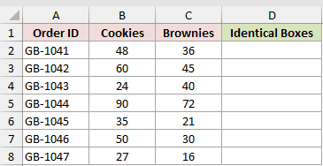
The goal is to find the largest number of identical boxes that can divide both quantities evenly.
Here is the formula entered in D2 and copied down:
=GCD(B2,C2)
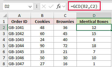
For order GB-1041, the quantities 48 and 36 return 12 identical boxes. Each row uses its own pair of values from columns B and C.
Order GB-1047 returns 1. Those quantities are coprime, so the order cannot be divided into more than one identical box.
Example 2: Calculate Row-by-Row GCDs With MAP
For board cutting, the calculation changes because each row needs its own answer.
Below is the dataset. Columns B and C contain paired board lengths. The row results belong in column D, while the pooled cell shows the wrong-way comparison.
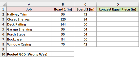
Each board pair needs its own greatest common divisor.
Here is the MAP formula:
=MAP(B2:B8,C2:C8,LAMBDA(a,b,GCD(a,b)))
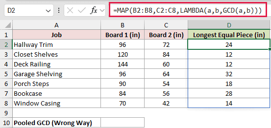
MAP passes each row’s two lengths to GCD, and the results spill from D2 through D8.
For Hallway Trim, 24 is the longest piece, in inches, that both the 96-inch and 72-inch boards can be cut into with no waste. Window Casing returns 14.
Here is the pooled GCD formula shown as the wrong-way comparison:
=GCD(B2:B8,C2:C8)
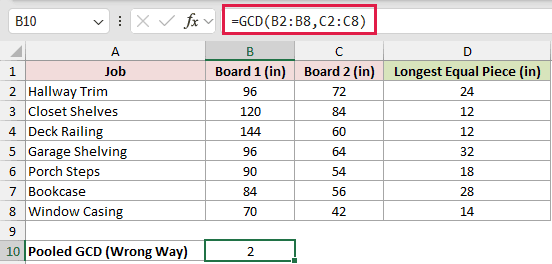
The white comparison cell returns 2 because GCD pools every number from both ranges into one calculation. It does not calculate the board pairs row by row.
Pro Tip: MAP is available in Microsoft 365 and Excel 2024. In other versions, use the filled-down approach from Example 1 for row pairs.
Example 3: Simplify Screen Aspect Ratios
Screen dimensions show how GCD preserves an exact ratio.
Below is the dataset. It lists each monitor location with its width and height in pixels. The Aspect Ratio column is reserved for the simplified result.
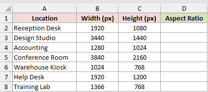
We want to divide both dimensions by their GCD and join the reduced values with a colon.
Here is the formula entered in D2 and copied down:
=B2/GCD(B2,C2)&":"&C2/GCD(B2,C2)
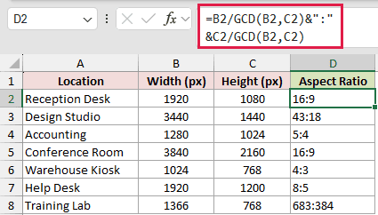
GCD finds the shared divisor. The formula divides the width and height by that value, then joins the reduced parts as text.
The 1920 by 1080 screen reduces to 16:9. However, the 1366 by 768 screen reduces exactly to 683:384, not 16:9.
That last result matters when you need the exact pixel ratio rather than a rounded marketing label.
Example 4: Simplify a Three-Part Ratio
The same method can reduce three quantities together.
Below is the dataset. Each store has Small, Medium, and Large order quantities. The Size Ratio column is where the reduced three-part result will appear.
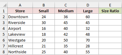
Each store needs one simplified size ratio.
Here is the formula entered in E2 and copied down:
=TEXTJOIN(":",TRUE,B2:D2/GCD(B2:D2))
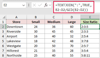
GCD pools the values across B2:D2 and returns their shared divisor. Dividing the row by that value reduces every part together.
TEXTJOIN then combines the reduced values with colons. Downtown’s quantities 24, 36, and 60 become 2:3:5.
TEXTJOIN itself is available in Excel 2019, Excel 2021, Excel 2024 and Microsoft 365.
The formula is copied down because each store needs a separate GCD from its own row.
Example 5: Find a Shared Carton Size
A carton-sizing problem uses one GCD for the entire range.
Below is the dataset. It lists products and units ordered. The Cartons Needed column and a separate result cell are ready for the calculations.
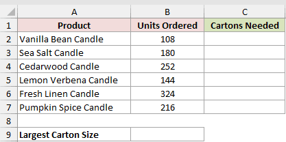
We want the largest carton size that divides every order, then the required carton count for each product.
Here is the formula for the largest carton size:
=GCD(B2:B7)
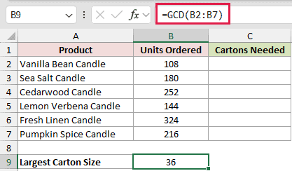
The formula pools every quantity in B2:B7 and returns 36 in B9. That is the largest carton size shared by every order.
Now divide each order quantity by the carton size:
=B2:B7/B9
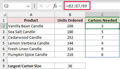
This range formula spills the carton counts into C2:C7 in Excel 2021, Excel 2024 and Microsoft 365. Earlier versions need a per-row formula copied down.
The 108-unit order needs 3 cartons, while the 324-unit order needs 9. No order leaves a partial carton.
If leftovers are allowed, QUOTIENT can count only the full cartons instead.
Example 6: Handle Decimals, Zeros, and Errors
The last example checks several inputs that often cause surprises.
Below is the dataset. Each scenario supplies two inputs, and the GCD column will show the result or the deliberate error returned for that row.
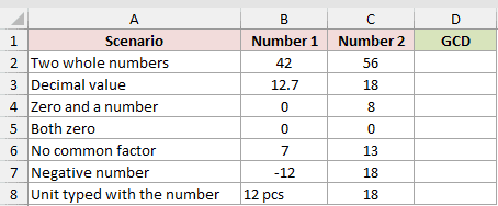
This time, the goal is to see how the same GCD formula handles each input pair.
Here is the formula entered in D2 and copied down:
=GCD(B2,C2)
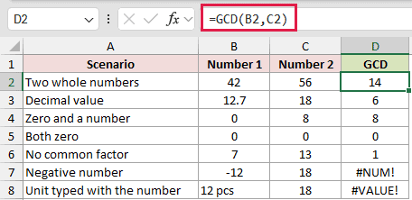
The whole numbers 42 and 56 return 14. Excel truncates the decimal in 12.7 before calculating with 18, so that row returns 6.
GCD returns 8 for 0 and 8, while two zeros return 0. The coprime pair 7 and 13 returns 1.
The final rows deliberately demonstrate errors. A negative input returns #NUM!, while the text value “12 pcs” returns #VALUE!.
Tips & Common Mistakes
- A GCD range formula pools all included numbers into one result. Use MAP in Microsoft 365 or Excel 2024 when you need paired row results from one spilling formula.
- Excel truncates decimals before calculating GCD. Check or clean decimal inputs if dropping the fractional part would hide a data problem.
- Negative inputs return #NUM!, and text such as “12 pcs” returns #VALUE!. Keep units in a separate cell from the number.
- A result of 1 means the numbers are coprime. They share no larger whole-number divisor.
- Use LCM when you need the least common multiple instead of the greatest shared divisor.
Passing an entire range to GCD returns one shared divisor. Row-level comparisons need a per-row formula or MAP instead.
That scope choice determines whether Excel groups the full dataset or calculates each pair separately.
Related Excel Functions / Articles:
