
Excel’s MAP function applies a LAMBDA calculation to each value in an array, or to corresponding values in multiple arrays.
It is useful for custom calculations that need to run once per item. When several arrays are supplied, each LAMBDA parameter represents the corresponding item from one array.
In this article, I’ll show you how to calculate from multiple arrays, test conditions row by row, and clean text across a range.
MAP Function Syntax in Excel
The MAP function takes one or more arrays and passes their values to a LAMBDA function that returns one result for each position.
=MAP(array1, lambda_or_array<#>)
array1is the first array whose values you want to map.lambda_or_array<#>represents any additional arrays followed by the LAMBDA calculation. The LAMBDA must be the final argument and have one parameter for each array supplied.
When to Use the MAP Function
- Apply a custom calculation to every value in a range without filling a formula down.
- Combine corresponding values from two or more arrays.
- Test several conditions separately for each row.
- Build a Boolean include array for another dynamic array function.
- Clean or standardize each text value in a list.
Example 1: Apply a Calculation to a Two-Dimensional Array
Let’s start by adjusting a full block of service volumes at once.
Below is the dataset with five service queues and their volumes for Monday through Wednesday.
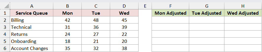
I want to increase every value by 10% and round the adjusted volumes to whole numbers.
Here is the formula:
=MAP(B2:D6,LAMBDA(t,ROUND(t*1.1,0)))
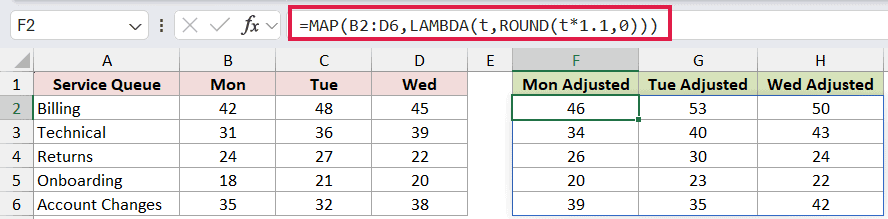
MAP passes each value from B2:D6 to the LAMBDA parameter t. The calculation multiplies that value by 1.1, rounds it to zero decimal places, and returns a five-row by three-column result starting in F2.
Pro Tip: For simple arithmetic, =ROUND(B2:D6*1.1,0) is shorter. MAP becomes more useful when the calculation is complex or when you want the logic clearly named inside LAMBDA.
Example 2: Calculate Labor Costs from Two Arrays
Now let’s pair values from two columns.
Below is the dataset with six work orders, their labor hours, and the hourly rate for each order.
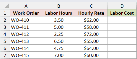
I want to multiply each work order’s hours by its corresponding hourly rate.
Here is the formula:
=MAP(B2:B7,C2:C7,LAMBDA(hours,rate,hours*rate))
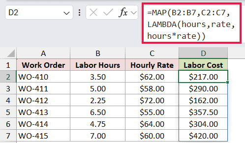
The first LAMBDA parameter, hours, receives values from B2:B7. The second, rate, receives the matching values from C2:C7. Excel multiplies each pair and spills the six labor costs from D2 to D7.
For example, WO-410 costs $217 because 3.5 hours multiplied by $62 equals $217.
Example 3: Test Two Conditions Row by Row
Here’s a useful way to evaluate paired TRUE and FALSE values.
Below is the dataset with seven applications and two checks for each one: whether the ID was verified and whether the agreement was signed.
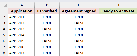
I want a TRUE result only when both checks are TRUE for the same application.
Here is the formula:
=MAP(B2:B8,C2:C8,LAMBDA(id,terms,AND(id,terms)))
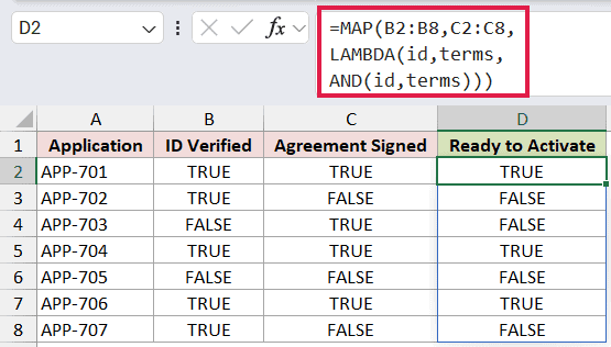
MAP sends the two values from each row to the AND function. AND returns TRUE only when both are TRUE, so APP-701, APP-704, and APP-706 pass both checks.
The formula spills one result per application, making the row-by-row relationship easy to see.
Example 4: Use MAP Inside FILTER
Let’s use MAP to create the include test for another formula.
Below is the dataset with vendor names, risk scores, and review statuses.
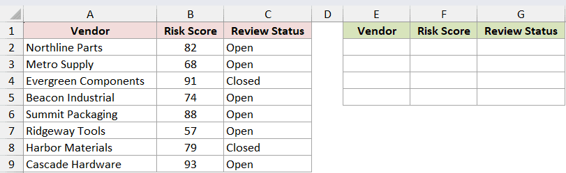
I want to return only vendors whose risk score is at least 70 and whose status is Open.
Here is the formula:
=FILTER(A2:C9,MAP(B2:B9,C2:C9,LAMBDA(score,status,AND(score>=70,status="Open"))),"No matches")
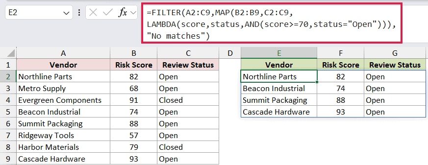
MAP tests each score and status pair, producing a TRUE or FALSE include array. FILTER uses that array to return Northline Parts, Beacon Industrial, Summit Packaging, and Cascade Hardware.
The final "No matches" argument supplies a readable message if no vendor meets both conditions.
Pro Tip: In this case, =FILTER(A2:C9,(B2:B9>=70)*(C2:C9="Open"),"No matches") is more direct. The MAP version is worth knowing when the include test needs custom LAMBDA logic.
Example 5: Clean and Standardize Text Values
MAP is also handy when each text value needs the same cleanup steps.
Below is the dataset with seven customer service IDs and team codes that contain blanks, extra spaces, and inconsistent capitalization.
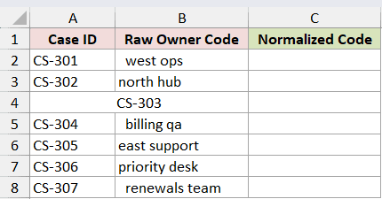
I want a consistent uppercase code with hyphens, while labeling blank entries as Unassigned.
Here is the formula:
=MAP(B2:B8,LAMBDA(code,IF(code="","Unassigned",UPPER(SUBSTITUTE(TRIM(code)," ","-")))))
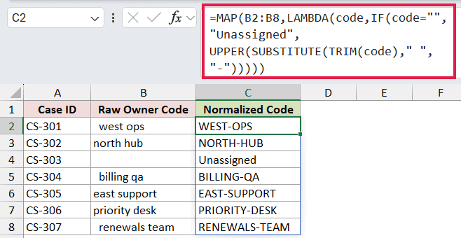
For each value, IF checks whether the code is blank. If it is not, TRIM removes unwanted spaces, SUBSTITUTE changes the remaining spaces to hyphens, and UPPER changes the result to uppercase.
The results spill from C2 to C8. The blank third code becomes Unassigned, while west ops becomes WEST-OPS.
Example 6: Calculate a Running Average with MAP
Finally, let’s use MAP to calculate an expanding result.
Below is the dataset with response times for seven consecutive weeks.
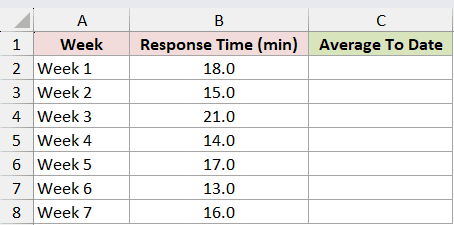
I want each row to show the average response time from Week 1 through that week.
Here is the formula:
=MAP(SEQUENCE(ROWS(B2:B8)),LAMBDA(n,AVERAGE(TAKE(B2:B8,n))))
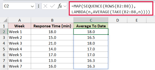
SEQUENCE creates the positions 1 through 7. For each position n, TAKE returns the first n response times and AVERAGE calculates their mean.
The spilled results start at 18.0 minutes for Week 1 and end at 16.3 minutes for Week 7.
Pro Tip: SCAN is usually the cleaner choice for a running calculation. One alternative is =SCAN(0,B2:B8,LAMBDA(total,value,total+value))/SEQUENCE(ROWS(B2:B8)), which builds a running sum and divides it by each position.
Tips & Common Mistakes
- MAP is available in Excel for Microsoft 365 and Excel 2024 for Windows and Mac. Earlier perpetual versions do not support it.
- Keep the mapped arrays the same size and shape so corresponding values line up as intended.
- Give the LAMBDA one parameter for every array passed to MAP. A mismatch returns a #VALUE! error labeled Incorrect Parameters.
- Enter a MAP formula once in its anchor cell. Do not fill it down because the returned array spills automatically.
- Make sure the intended spill range is empty. Existing values in that area cause a #SPILL! error.
I use MAP when a calculation is easiest to express as a small, named operation applied to every array position. The six examples above cover one array, paired arrays, Boolean tests, filtering, text cleanup, and an expanding calculation.
I hope you found this article helpful.
Related Excel Functions / Articles:
