
Excel’s HARMEAN function returns the harmonic mean of positive numbers. It calculates the reciprocal of the arithmetic mean of their reciprocals.
HARMEAN is useful for averaging rates when each rate covers the same distance, investment, or other numerator amount. Unlike AVERAGE, it gives more weight to smaller values.
In this article, I’ll show you how to calculate average speed, find average investment cost, and avoid misleading results when weights or rates differ.
HARMEAN Function Syntax in Excel
The HARMEAN function accepts from 1 to 255 numeric arguments.
=HARMEAN(number1, [number2], ...)
- number1 (required) is the first positive number, cell reference, range, array, or name you want to include.
- number2, … (optional) are additional positive numbers, references, ranges, arrays, or names you want to include.
When to Use HARMEAN Function
- Calculate average speed when every leg covers the same distance.
- Find average cost per share when you invest the same amount each period.
- Average ratios such as P/E values when the underlying allocations are equal.
- Combine precision and recall into an F1 score.
- Calculate a conditional harmonic mean after filtering a range.
Example 1: Calculate Average Speed Over Equal Laps
Let’s start with bike laps that all cover the same distance.
Below is the dataset. Columns A to C list eight five-mile laps and their speeds. The result card contains three labeled empty cells under a green header.
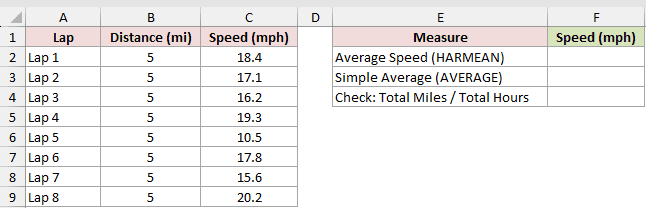
First, we want the true average speed across all eight equal-distance laps.
Here is the formula:
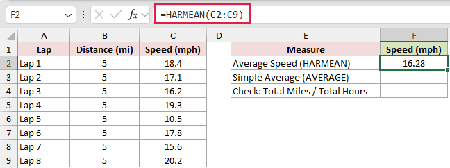
=HARMEAN(C2:C9)
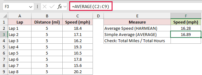
For comparison, this formula calculates the simple average of the lap speeds:
=AVERAGE(C2:C9)
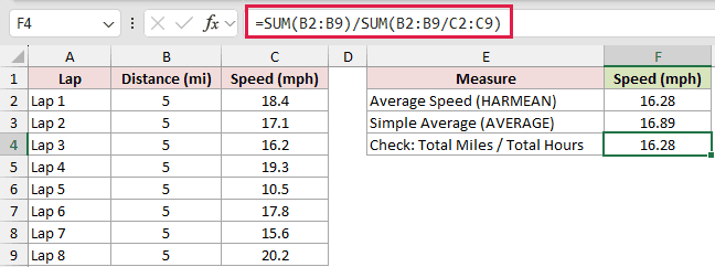
We can also divide total distance by total riding time to check the result:
=SUM(B2:B9)/SUM(B2:B9/C2:C9)
The array division inside SUM can be entered normally in Excel 2021, Excel 2024, and Microsoft 365. Excel 2019 and earlier require Ctrl+Shift+Enter.
HARMEAN returns 16.28 mph, while AVERAGE returns 16.89 mph. The 10.5 mph lap pulls the harmonic mean down more strongly.
The total-distance divided by total-time formula also returns 16.28 mph. That match confirms HARMEAN works here because every lap covers five miles.
Example 2: Find Average Cost per Share
Here’s a fixed-investment example with prices that rise and fall.
Below is the dataset. Columns A to C show ten monthly $300 investments and the share price. The result card has two labeled empty cells under a green header.
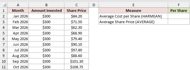
We want to calculate the investor’s average cost per share and compare it with the average market price.
Here is the average cost formula:
=HARMEAN(C2:C11)
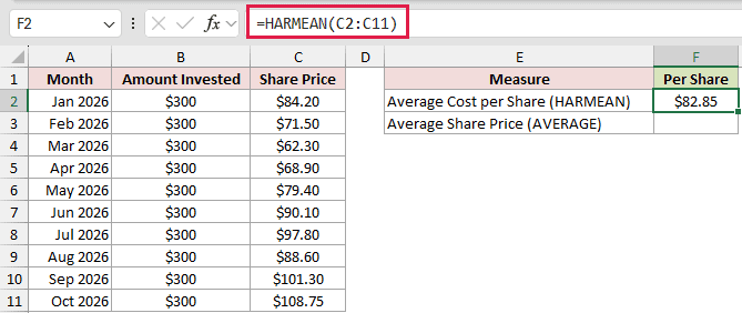
Here is the simple average price for comparison:
=AVERAGE(C2:C11)
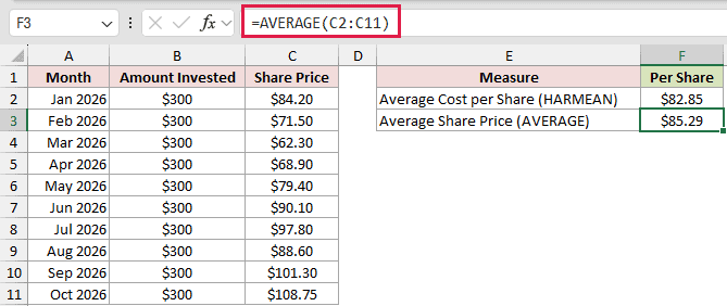
HARMEAN returns an average cost of $82.85 per share. AVERAGE returns $85.29 for the same price list.
The harmonic mean fits because every monthly contribution is $300. Lower prices buy more shares, so they have more influence on the investor’s cost per share.
Example 3: Handle Unequal Spending Amounts
Now let’s see what changes when the amounts aren’t equal.
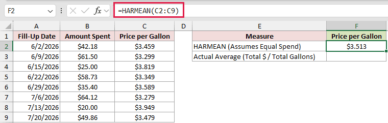
Below is the dataset. Columns A to C list eight fuel purchases with different amounts and prices. The result card shows two labeled empty cells under a green header.
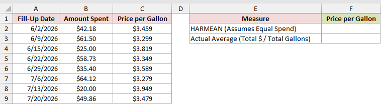
We want to check whether an unweighted HARMEAN reflects the actual average price paid per gallon.
Here is the unweighted harmonic mean:
=HARMEAN(C2:C9)
Here is the actual average, calculated as total spending divided by total gallons purchased:
=SUM(B2:B9)/SUM(B2:B9/C2:C9)
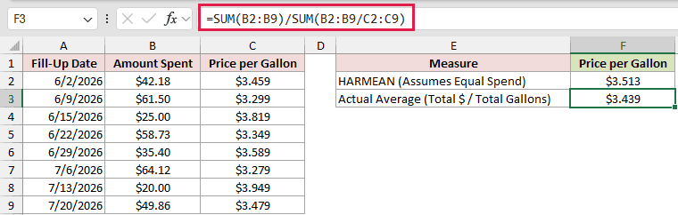
HARMEAN assumes the same dollar amount was spent at each price and returns $3.513. The purchases vary from $20.00 to $64.12, so that assumption doesn’t fit.
The weighted calculation returns the actual average of $3.439 per gallon. The array expression B2:B9/C2:C9 returns one gallon amount per row before SUM adds them up.
Pro Tip: For unequal amounts, the general weighted pattern is =SUM(amounts)/SUM(amounts/rates).
Example 4: Calculate Harmonic Mean by Sector
Here’s a practical way to calculate a separate result for each group.
Below is the dataset. Columns A to C list 12 companies, sectors, and P/E ratios.
Columns E and F show the Sector and green Average P/E headers, sector labels, and empty result cells.
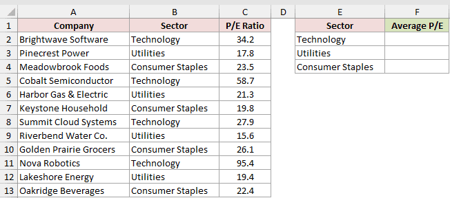
We want to calculate the harmonic mean P/E ratio for each sector.
Here is the formula entered in F2 and copied down through F4:
=HARMEAN(FILTER($C$2:$C$13,$B$2:$B$13=E2))
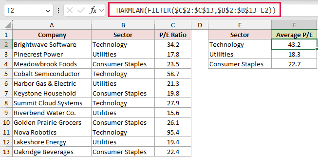
FILTER returns the P/E ratios for the sector named in column E. HARMEAN then reduces that filtered array to one value.
The results are 43.2 for Technology, 18.3 for Utilities, and 22.7 for Consumer Staples. Technology’s simple average would be 54.05 because of the 95.4 ratio.
The harmonic mean P/E is the P/E of an equal-dollar allocation across the companies in each sector.
FILTER requires Excel 2021, Excel 2024, or Microsoft 365.
Example 5: Calculate F1 Scores
Let’s use HARMEAN to combine precision and recall into an F1 score for each filter version.
Below is the dataset. Columns A to C list six versions with precision and recall.
The two result columns have empty bordered cells under the green “F1 Score (HARMEAN)” and “Simple Average” headers.
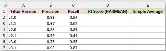
We want to calculate each version’s F1 score and compare it with the simple average of precision and recall.
Here is the formula entered in D2 and copied down through D7:
=HARMEAN(B2,C2)
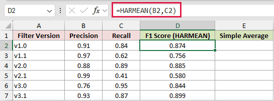
Here is the comparison formula entered in E2 and copied down through E7:
=AVERAGE(B2,C2)
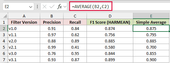
For v1.0, the HARMEAN formula returns an F1 score of 0.874, and the AVERAGE formula returns 0.875 because the two measures are close.
Version v2.1 has 0.99 precision but only 0.41 recall. Its F1 score is 0.580, well below the 0.700 simple average.
The harmonic mean penalizes that imbalance, so one strong measure can’t hide a weak one.
Example 6: Fix #NUM! Errors From Zeros
The last example shows why one zero can stop the whole calculation.
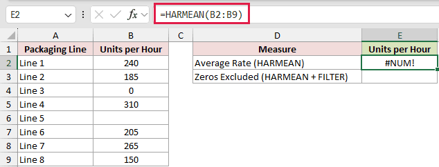
Below is the dataset. Columns A and B list eight packaging lines, with one zero rate and one blank.
The result card has a green Units per Hour header and two labeled empty cells.
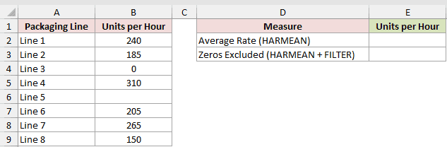
We want to see the original error and then average only the lines with positive reported rates.
For this example, assume each line handles the same number of units, so HARMEAN is the right average.
Here is the formula that includes the zero:
=HARMEAN(B2:B9)
Here is the formula that keeps only positive rates:
=HARMEAN(FILTER(B2:B9,B2:B9>0))
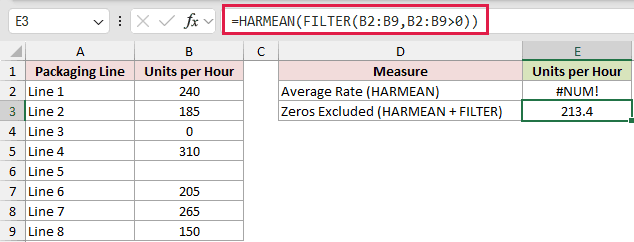
The first formula returns #NUM! because B4 contains zero. The blank cell in B6 is ignored and doesn’t cause the error.
FILTER leaves six positive reported rates, so HARMEAN returns 213.4 units per hour for those six lines. The zero in B4 and unreported blank in B6 are excluded.
If every line ran for the same number of hours, AVERAGE would be the right combined rate.
FILTER requires Excel 2021, Excel 2024, or Microsoft 365.
Pro Tip: Excluding zeros changes the meaning of the result. Confirm that your reporting rules allow you to exclude a zero.
Tips & Common Mistakes
- HARMEAN accepts positive values only. Any zero or negative number in the calculation returns #NUM!.
- Text, logical values, and blanks inside a referenced range are ignored. A direct nonnumeric text argument returns #VALUE!.
- Use HARMEAN only when the underlying amounts have equal weight. Unequal distances, spending amounts, or quantities need a weighted harmonic mean.
- For positive values, HARMEAN can’t exceed GEOMEAN, and GEOMEAN can’t exceed AVERAGE.
- If precision or recall is zero, HARMEAN returns #NUM!, although the conventional F1 score is zero. Handle that case explicitly before applying HARMEAN.
- In Excel 2021, Excel 2024, or Microsoft 365, HARMEAN returns one value but can summarize a spilled range with
=HARMEAN(A2#). - In Excel 2024 or Microsoft 365,
=BYROW(B2:C7,LAMBDA(r,HARMEAN(r)))can spill all F1 scores instead of using a fill-down formula.
The AVERAGE comparisons make the effect of smaller values easy to see.
FILTER also lets HARMEAN work with one group or a chosen set of positive rates.
Related Excel Functions / Articles:
