
Excel’s DPRODUCT function returns the product of numeric values in a database field for records that match a criteria range.
Unlike PRODUCT, DPRODUCT can restrict the multiplication to records that match the criteria.
It works well for combining probabilities, yields, growth factors, or multipliers when the product has a practical meaning.
In this article, I’ll show you how to compound matching values, build AND and OR criteria, avoid text-matching traps, and handle empty results.
DPRODUCT Function Syntax in Excel
The DPRODUCT function uses a database, a field to multiply, and a worksheet criteria range.
=DPRODUCT(database, field, criteria)
- database (required) is the full list or range, including its column headers.
- field (required) identifies the column to multiply. Use its header in quotation marks, a cell containing the header, or its column position within the database.
- criteria (required) is a range containing at least one copied database header and a condition below it.
Criteria on the same row use AND logic. Criteria on separate rows use OR logic.
When to Use DPRODUCT Function
- Multiply probabilities or process yields only for records that match a category.
- Compound growth factors for one account, property, product, or time period.
- Combine several pricing multipliers selected by worksheet criteria.
- Keep criteria visible in cells so someone can change them without editing the formula.
Example 1: Multiply Matching On-Time Rates
Let’s start with one text criterion and a meaningful product.
Below is the dataset. Columns A to D list orders and on-time rates. F1:F2 holds the Kitchen Remodel criterion. H2 is an empty bordered answer cell under its green header.
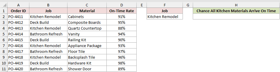
We want the chance that every material for the Kitchen Remodel arrives on time.
Here is the formula:
=DPRODUCT(A1:D11,"On-Time Rate",F1:F2)
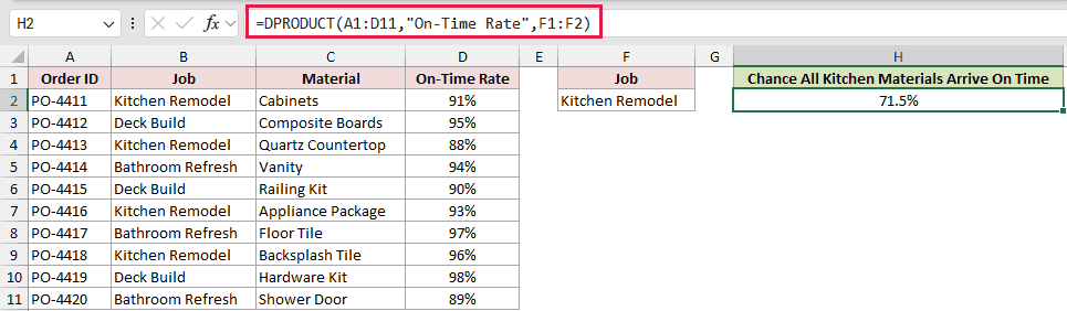
DPRODUCT finds the four Kitchen Remodel rows and multiplies their on-time rates. The result is 71.5%, which is lower than any single rate in the group.
This interpretation assumes the vendors’ delays are independent. If one delay makes another more likely, multiplying the rates doesn’t give a reliable joint probability.
Example 2: Compound Rent Increases With AND Criteria
Here’s a compounding example with two conditions.
Below is the dataset. Columns A to D hold property increases and factors. F1:G2 selects Maple Court from 2023 onward. I2 is empty and bordered under its green header.
The Increase Factor column is already filled with =1+C2 copied down, so each percentage becomes a value that DPRODUCT can compound.
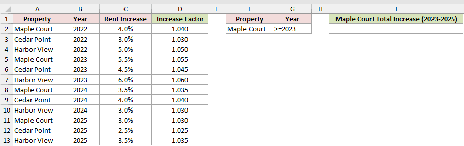
We want Maple Court’s total rent increase from 2023 through 2025.
Here is the formula:
=DPRODUCT(A1:D13,"Increase Factor",F1:G2)-1
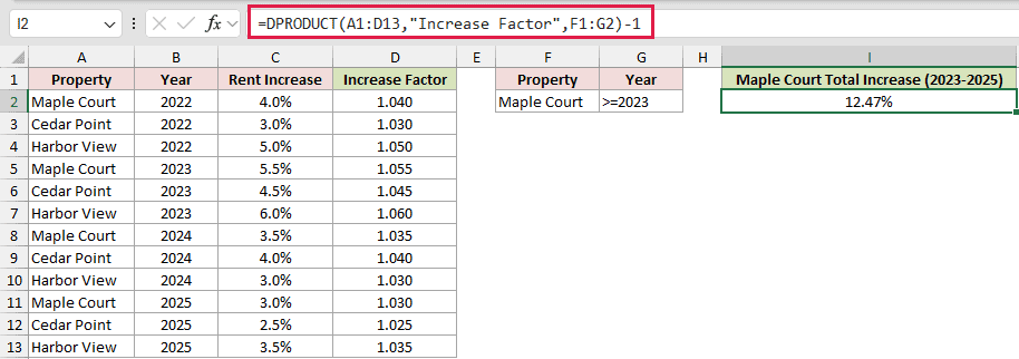
Both criteria sit on one row, so Excel matches Property values beginning with Maple Court AND Year values of at least 2023.
DPRODUCT multiplies the three factors, then subtracts 1. The compounded increase is 12.47%, about 0.47 percentage points above the 12% found by adding the rates.
The gap is small over three years.
In Excel 2021, Excel 2024, or Microsoft 365, =PRODUCT(1+FILTER(C2:C13,(A2:A13="Maple Court")*(B2:B13>=2023)))-1 produces the result without a helper factor column.
Example 3: Calculate Yield With OR Criteria
Now let’s use two criteria rows to include different kinds of process steps.
Below is the dataset. Columns A to D list production steps and yields. F1:F3 contains All Models and Kayak. H2 is empty and bordered under its green header.
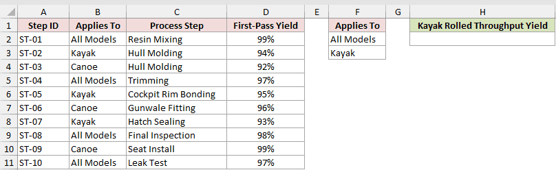
We want the rolled throughput yield for every shared step or Kayak-only step.
Here is the formula:
=DPRODUCT(A1:D11,"First-Pass Yield",F1:F3)
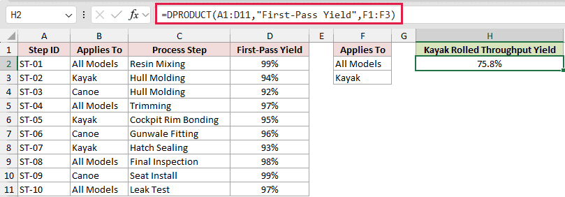
The two conditions appear on separate criteria rows, so they use OR logic. Excel includes rows labeled All Models or Kayak.
Multiplying the seven matching yields returns 75.8%. This is the share expected to pass every included step on the first attempt.
Example 4: Force an Exact Text Match
This example shows a text-matching detail that can quietly change the result.
Below is the dataset. Columns A to D list pricing layers. F1:F2 holds Channel and Online, while H1:H2 holds Channel and the exact-match criterion.
The formula ="=Online" already appears in H2 as criteria data. J2 and K2 are empty bordered answer cells under their green headers, positioned side by side.
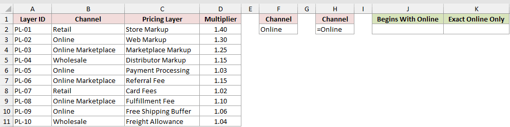
We want to compare a plain Online criterion with a criterion that matches Online exactly.
First, use the plain criterion in F1:F2:
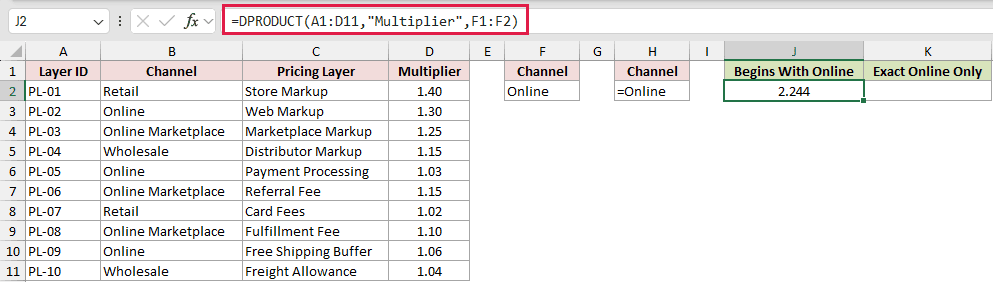
=DPRODUCT(A1:D11,"Multiplier",F1:F2)
Now use the exact-match criterion in H1:H2:
=DPRODUCT(A1:D11,"Multiplier",H1:H2)
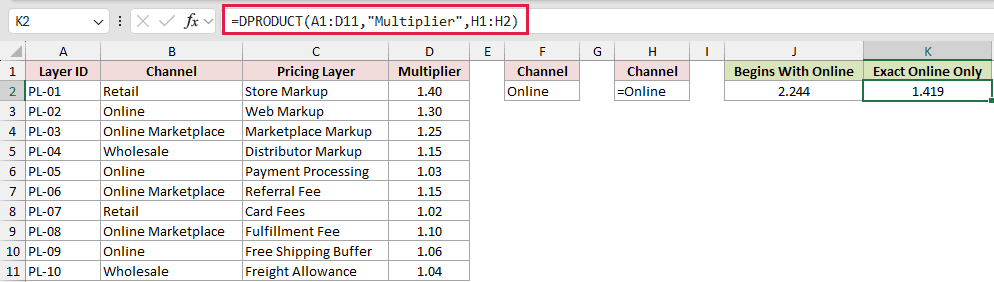
The plain Online criterion acts as a begins-with match. J2 returns 2.244 because Excel includes both Online and Online Marketplace layers.
The exact criterion returns 1.419 in K2. It multiplies only the three rows whose Channel is exactly Online.
Pro Tip: For an exact text match, put ="=Online" in the criteria value cell. A plain Online criterion also matches text that begins with Online.
Example 5: Handle DPRODUCT’s No-Match Result
This example uses a criterion that matches no rows.
Below is the dataset. Columns A to D list nursery batches and survival rates. F1:F2 asks for Kale. H2:I2 holds two empty bordered answer cells under green headers.
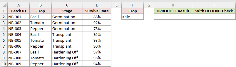
We want to compare DPRODUCT’s result with a guarded formula when no Kale records exist.
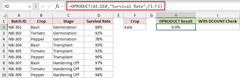
Here is the DPRODUCT formula:
=DPRODUCT(A1:D10,"Survival Rate",F1:F2)
Now add a DCOUNT check before calculating the product:
=IF(DCOUNT(A1:D10,"Survival Rate",F1:F2)=0,"No records",DPRODUCT(A1:D10,"Survival Rate",F1:F2))
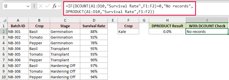
No rows match Kale, but DPRODUCT returns 0.0% instead of an error. That result can look like a genuine zero survival rate.
The guarded formula uses DCOUNT to test for matching numeric records first. It returns No records, which makes the missing group clear.
Pro Tip: Use a DCOUNT check when an empty match could be mistaken for a real zero. DPRODUCT doesn’t distinguish those cases for you.
Example 6: Use PRODUCT With FILTER by Group
The last example uses a modern formula instead of a database criteria range.
Below is the dataset. Columns A to C list annual fund returns. E2:E4 contains the fund names. The empty bordered cells F2:F4 sit under the single green “Cumulative Return (2022-2025)” header.
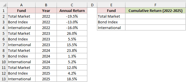
We want the cumulative return for each fund from 2022 through 2025.
Here is the formula entered in F2 and copied down:
=PRODUCT(1+FILTER($C$2:$C$13,$A$2:$A$13=E2))-1
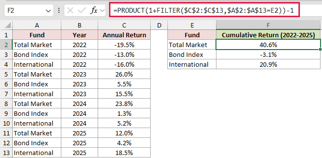
FILTER returns the annual rates for the fund named in column E. Adding 1 creates growth factors, PRODUCT compounds them, and subtracting 1 restores a return.
The results are 40.6% for Total Market, -3.1% for Bond Index, and 20.9% for International.
This approach needs Excel 2021, Excel 2024, or Microsoft 365. DPRODUCT works in older versions, but it needs a worksheet criteria range and a factor column for rates.
Tips & Common Mistakes
- Copy database headers exactly into the criteria range. A misspelled field argument returns
#VALUE!, while field names are not case-sensitive. - Put conditions side by side on one criteria row for AND logic. Stack conditions on separate rows for OR logic.
- Plain text criteria use begins-with matching. Use a criteria formula such as
="=Online"when you need the whole text to match exactly. - DPRODUCT returns 0 when no records match. Check with DCOUNT when zero could be confused with a valid result.
- Blank and text cells in the field are skipped. Compare DCOUNT with the number of expected records when missing values could overstate a probability or yield.
- Use PRODUCT when every value should be included. For modern conditional calculations, PRODUCT and FILTER often avoid the separate worksheet criteria range.
- DPRODUCT returns one value rather than spilling. It can still use a spilled criteria range such as
F1#, but that needs Excel 2021, Excel 2024, or Microsoft 365.
DPRODUCT can combine matching probabilities, yields, increases, and multipliers through visible worksheet criteria.
Build the criteria carefully, convert rates to factors, and check for empty matches before you trust the result.
Related Excel Functions / Articles:
