
Excel’s PRODUCT function multiplies numbers and returns their product. It accepts individual values, cell references, and ranges in the same formula.
That makes long multiplication chains easier to maintain. You can also combine it with array formulas to multiply selected values or compound a series of growth factors.
In this article, I’ll show you how to multiply ranges, compound growth rates, and multiply only values from matching rows.
PRODUCT Function Syntax in Excel
The PRODUCT function accepts numbers, cell references, ranges, or a mix of these arguments.
=PRODUCT(number1, [number2], ...)
- number1 (required) is the first number, cell reference, or range you want to multiply.
- number2 (optional) is another number, cell reference, or range. You can supply up to 255 arguments in modern Excel versions.
When to Use PRODUCT Function
- Multiply every numeric value in a range without writing a long chain of asterisk operators.
- Compound a series of growth rates or percentage changes by multiplying their growth factors.
- Ignore blanks, text, and logical values stored inside a referenced range while multiplying its numeric values.
- Combine PRODUCT with FILTER when you need to multiply only the rows that meet a condition.
- Combine a referenced range with a fixed adjustment in one multiplication formula.
Example 1: Multiply a Range With PRODUCT
Let’s start with a packing calculation that has several levels.
Below is the dataset. Column A lists four packing levels, while column B gives the quantity used at each level.
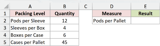
We want to calculate the number of coffee pods on one pallet.
Here is the formula:
=PRODUCT(B2:B5)
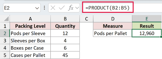
The formula multiplies 12 pods per sleeve, 4 sleeves per box, 6 boxes per case, and 45 cases per pallet.
The result is 12,960 pods per pallet. PRODUCT is easier to read than a long chain of separate cell references, especially when the range grows.
Example 2: Compound Yearly Growth Rates
Now let’s combine several positive and negative yearly growth rates.
Below is the dataset. Column A lists the years from 2020 through 2025, and column B contains the growth rate for each year.
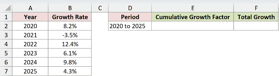
We want to calculate both the cumulative growth factor and the total growth across all six years.
Here is the formula for the cumulative growth factor:
=PRODUCT(1+B2:B7)
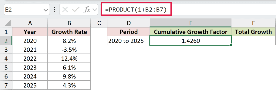
This formula adds 1 to every rate, turning each percentage into a growth factor before multiplying the six factors together.
The result is 1.4260. That factor tells us the ending value is 1.426 times the starting value.
To show the same change as a percentage, subtract 1 from the product:
=PRODUCT(1+B2:B7)-1
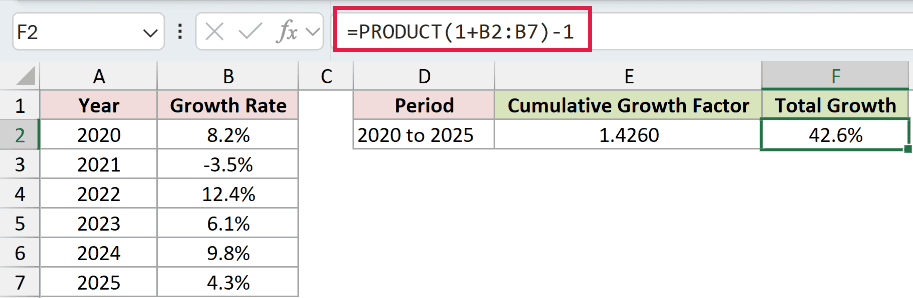
The second formula returns 42.6%, which is the total growth across the full period.
You cannot add yearly percentage changes because each new rate applies to the value produced by the previous year. Multiplying growth factors handles that compounding correctly.
Pro Tip: In Microsoft 365, Excel 2024, and Excel 2021, enter these formulas normally. In Excel 2019 and earlier, formulas using 1+B2:B7 require Ctrl+Shift+Enter.
Example 3: PRODUCT Versus the Asterisk Operator
Here’s where PRODUCT behaves better than a basic multiplication chain.
Below is the dataset. Column A lists freight surcharge steps, while column B contains four numeric multipliers, one blank, and the text value Waived.
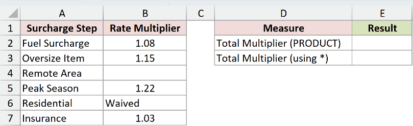
We want to multiply the usable numeric multipliers without cleaning the range first.
Here is the PRODUCT formula:
=PRODUCT(B2:B7)
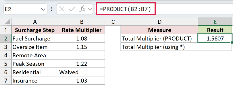
PRODUCT ignores the blank and the text stored inside the referenced range. It multiplies 1.08, 1.15, 1.22, and 1.03 to return 1.5607.
Now compare that with the asterisk operator:
=B2*B3*B4*B5*B6*B7
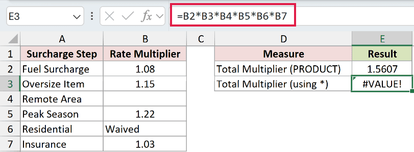
The second formula returns #VALUE! because it tries to multiply the text value Waived.
PRODUCT is not inherently faster than the asterisk operator. Use it here for its range-aware behavior, not as a performance optimization.
Pro Tip: The asterisk operator treats an empty cell as zero. Without the text error, that blank could quietly turn the entire multiplication result into 0.
Example 4: Multiply Only Matching Rows
Let’s add a condition by pairing PRODUCT with FILTER.
Below is the dataset. Columns A through C list discount codes, their price multipliers, and whether each code is Active or Expired.
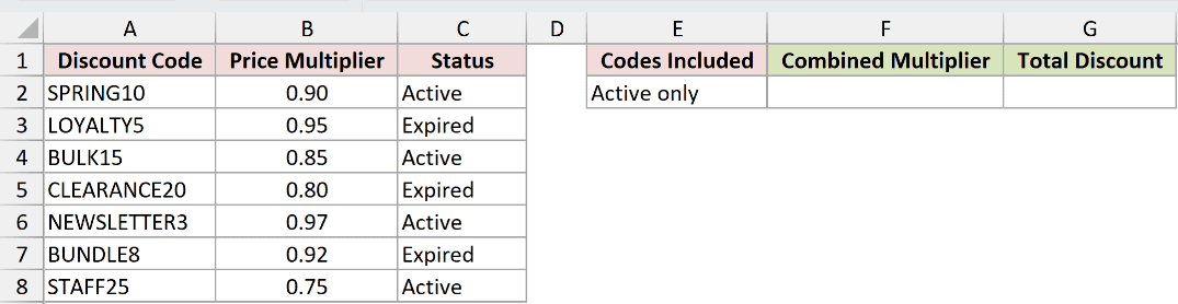
We want to multiply only the price multipliers belonging to active discount codes.
Here is the formula for the combined multiplier:
=PRODUCT(FILTER(B2:B8,C2:C8="Active"))
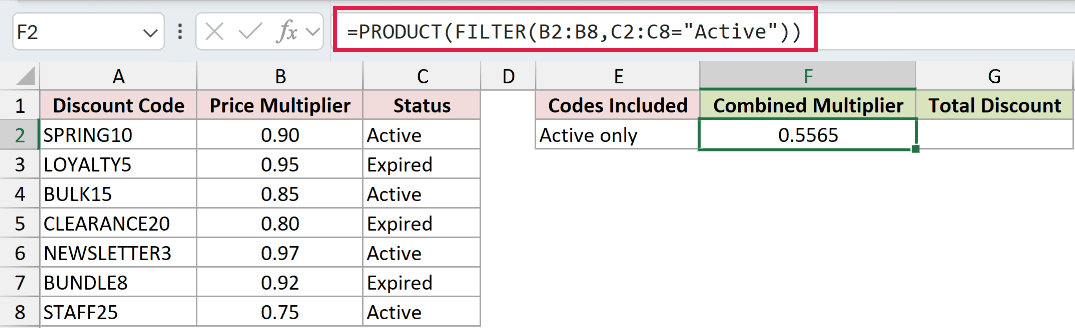
FILTER returns the multipliers from rows marked Active. PRODUCT then collapses that filtered array into the single result 0.5565.
To express the combined reduction as a percentage, subtract that multiplier from 1:
=1-PRODUCT(FILTER(B2:B8,C2:C8="Active"))
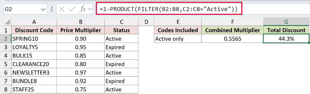
Multiplying the four active price multipliers gives a total discount of 44.3%.
PRODUCT has no PRODUCTIF or PRODUCTIFS companion. FILTER supplies the condition, while PRODUCT handles the multiplication.
Pro Tip: FILTER is available in Excel 365 and Excel 2021 or later. Older Excel versions need the classic IF array approach, confirmed with Ctrl+Shift+Enter.
Example 5: Mix a Range and Constant
Finally, let’s combine a range with a fixed contingency rate.
Below is the dataset. This parameter card contains hours per unit, units ordered, and the blended hourly rate.

We want to calculate the labor cost first, then include an 8% contingency in a second result.
Here is the labor cost formula:
=PRODUCT(B1:B3)
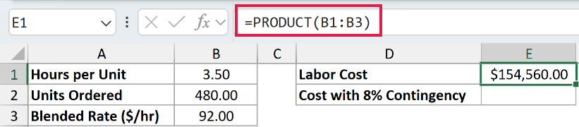
The formula multiplies 3.50 hours, 480 units, and a $92.00 hourly rate. It returns a labor cost of $154,560.00.
Now include the contingency as another PRODUCT argument:
=PRODUCT(B1:B3,1.08)
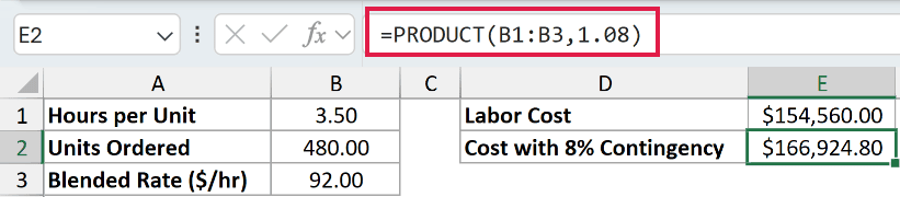
The second argument multiplies the base cost by 1.08. The result is $166,924.80 after adding the 8% contingency.
You could multiply the first result by 1.08 outside PRODUCT. Keeping the constant inside the function is a convenient style choice, not a different calculation.
Tips & Common Mistakes
- One zero anywhere in a referenced numeric range makes the entire product zero. Check unexpected zero results carefully because Excel does not flag them as errors.
- To multiply a spilled range, use its anchor, as in
=PRODUCT(D2#). Inside that array or reference, PRODUCT ignores blanks, text, and logical values. - PRODUCT returns one value, so it does not spill by itself. It can still consume an array returned by FILTER.
- Do not substitute PRODUCT for SUMPRODUCT.
=PRODUCT(B2:B8,C2:C8)multiplies all fourteen cells, while SUMPRODUCT multiplies aligned rows and adds the results. - In Excel 2019 and earlier, use
=PRODUCT(IF(C2:C8="Active",B2:B8))for conditional multiplication and confirm it with Ctrl+Shift+Enter.
PRODUCT keeps long multiplication chains readable and handles referenced blanks or text more gracefully than the asterisk operator.
Use it for straightforward range products, compounding, conditional multiplication, and calculations that mix ranges with fixed values.
Related Excel Functions / Articles:
