AMORDEGRC Function in Excel (4 Easy Examples)

The AMORDEGRC function in Excel returns depreciation for each accounting period under the French accounting system. It prorates the first period and applies a coefficient based on asset life.

Microsoft has deprecated AMORDEGRC because the French depreciation methodology changed. The function remains available only for compatibility with older workbooks and should not be used in new models.

In this article, I’ll show you how to maintain a legacy asset register, build a period schedule, understand coefficient bands, and compare AMORDEGRC with AMORLINC.

Table of Contents

AMORDEGRC Function Syntax in Excel

The AMORDEGRC function uses six required arguments and one optional argument:

=AMORDEGRC(cost, date_purchased, first_period, salvage, period, rate, [basis])

cost is the asset’s purchase cost.
date_purchased is the purchase date.
first_period is the end date of the first accounting period.
salvage is the asset’s value at the end of its useful life.
period is the accounting period for which you want depreciation. Period 0 is the prorated first period.
rate is the depreciation rate. Excel uses its reciprocal to determine the asset life and coefficient.
basis is optional. Use 0 or omit it for NASD 360, 1 for Actual, 3 for Actual/365, or 4 for European 360.

When to Use AMORDEGRC Function

Maintain an older workbook that already uses French coefficient depreciation.
Recalculate a legacy asset register after its input values change.
Trace a period-by-period schedule in an existing model.
Explain why AMORDEGRC and AMORLINC return different depreciation amounts.

Example 1: Maintain a Legacy Asset Register

Let’s start with several assets from an older depreciation file.

Below are four assets with purchase dates, first-period end dates, costs, salvage values, rates, bases, and periods. The Depreciation column is ready for formulas.

I want to calculate the depreciation amount for each asset and selected period.

Enter this formula in I2, then fill it down through I5:

=AMORDEGRC(D2,B2,C2,E2,H2,F2,G2)

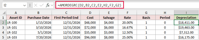
The formula passes one asset’s inputs to AMORDEGRC on each row. The saved results are $18,411.00, $19,463.00, $7,312.00, and $16,175.00.

Native Excel returned #VALUE! when these inputs were passed as plain ranges. The first-row formula is therefore filled down as separate scalar calculations.

Pro Tip: Keep AMORDEGRC only where an old workbook requires it. For a new model, choose a method that matches the current accounting policy.

Example 2: Build a Depreciation Schedule

A period schedule makes the function’s changing depreciation amounts easier to trace.

Below are periods 0 through 5 beside empty Depreciation and Ending Book Value columns. The asset card uses a $60,000 cost and zero salvage.

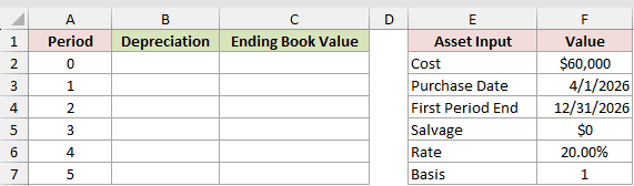
I first want to calculate depreciation for each period.

Enter this formula in B2, then fill it down through B7:

=AMORDEGRC($F$2,$F$3,$F$4,$F$5,A2,$F$6,$F$7)

=AMORDEGRC($F$2,$F$3,$F$4,$F$5,A2,$F$6,$F$7) in B2

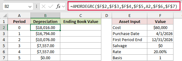
The absolute references keep the asset inputs fixed. The relative A2 reference advances from period 0 to period 5 as the formula is filled down.

Next, subtract period 0 depreciation from the original cost:

=$F$2-B2

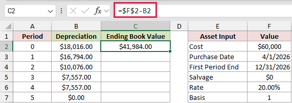
Cell C2 returns $41,984.00 after subtracting the first $18,016.00 depreciation charge from the $60,000 cost.

For later periods, subtract the current depreciation from the previous row’s ending book value:

=C2-B3

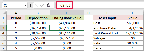
Enter the roll-forward formula in C3, then fill it down through C7. The ending book value reaches zero after period 4 because this example uses zero salvage.

The final depreciation sequence is $18,016, $16,794, $10,076, $7,557, $7,557, and $0.

Example 3: See the Coefficient Bands

AMORDEGRC changes its depreciation coefficient according to the asset life calculated as 1 / rate.

Below are useful lives of 4, 5, and 8 years with matching rates. A shared asset card supplies the other inputs.

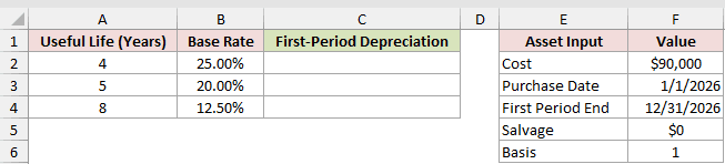
I want to compare first-period depreciation across the documented coefficient bands.

Enter this formula in C2, then fill it down through C4:

=AMORDEGRC($F$2,$F$3,$F$4,$F$5,0,B2,$F$6)

=AMORDEGRC($F$2,$F$3,$F$4,$F$5,0,B2,$F$6) in C2

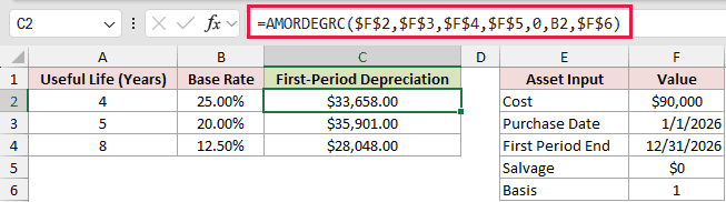
The relative B2 reference supplies each row’s base rate. The formula keeps the other asset inputs fixed and always calculates period 0.

Excel returns $33,658.00 at 25%, $35,901.00 at 20%, and $28,048.00 at 12.5%.

Microsoft documents coefficients of 1.5 for lives from 3 to 4 years, 2 for 5 to 6 years, and 2.5 for lives over 6 years.

Example 4: Compare AMORDEGRC and AMORLINC

The two French accounting functions use similar inputs but calculate depreciation differently.

Below is one asset card with empty result cells for AMORDEGRC and AMORLINC.

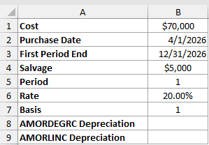
I first want to calculate period 1 depreciation with AMORDEGRC.

Here is the formula:

=AMORDEGRC(B1,B2,B3,B4,B5,B6,B7)

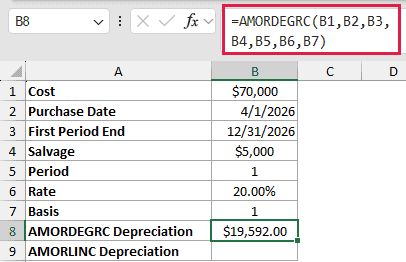
AMORDEGRC returns $19,592.00 because it applies the coefficient method.

Now calculate the same period with AMORLINC:

=AMORLINC(B1,B2,B3,B4,B5,B6,B7)

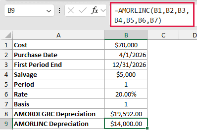
AMORLINC returns $14,000.00 because it uses a linear method. It is a useful comparison, but it is not a drop-in replacement for AMORDEGRC.

Pro Tip: Replacing AMORDEGRC changes the accounting method and results. Have the applicable policy confirmed before changing an old workbook.

Tips & Common Mistakes

Microsoft has deprecated AMORDEGRC and says it should no longer be used. It remains available for old-workbook compatibility.
Use real Excel dates or the DATE function. Text dates can cause errors.
Basis accepts 0, 1, 3, or 4. Basis 2 is not supported by this function.
Microsoft documents #NUM! for useful-life bands from 0 to 1, 1 to 2, 2 to 3, and 4 to 5 years.
Plain range arguments returned #VALUE! in native Excel testing. Use one scalar formula per row and fill down.
A book-value roll-forward needs a different first formula. Start with cost minus first depreciation, then subtract each later charge from the preceding balance.

I covered legacy asset calculations, a complete period schedule, coefficient bands, and the difference between AMORDEGRC and AMORLINC.

I hope you found this article helpful.