
The SYD function in Excel returns an asset’s sum-of-years’ digits depreciation for a specified period.
This accelerated method records more depreciation early in an asset’s life and less later. You still depreciate only the difference between its cost and salvage value.
In this article, I’ll show you how to calculate one period, build a complete depreciation schedule, and handle an asset purchased partway through a fiscal year.
SYD Function Syntax in Excel
The SYD function uses four required arguments in the following order.
=SYD(cost, salvage, life, per)
- cost is the asset’s original cost.
- salvage is the expected value at the end of the asset’s useful life.
- life is the number of periods over which the asset is depreciated.
- per is the period for which you want depreciation. It must use the same units as life.
When to Use SYD Function
- Calculate accelerated depreciation for a particular year of an asset’s useful life.
- Build a year-by-year depreciation schedule that records larger expenses in earlier years.
- Calculate current-year depreciation for several assets at different stages of their useful lives.
- Find accumulated depreciation and book value after a chosen number of years.
- Prorate SYD depreciation when an asset enters service partway through a fiscal year.
Example 1: Calculate SYD for One Year
We’ll begin with a single depreciation calculation.
Below is an input card for a $41,800 cargo van with $5,800 salvage, a five-year life, and Year 2 selected. The final row will hold the result.
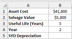
The goal is to calculate the van’s depreciation expense for its second year.
Here is the formula:
=SYD(B1,B2,B3,B4)
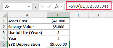
Cells B1 and B2 provide the cost and salvage value. B3 supplies the five-year life, while B4 tells SYD to return the Year 2 amount.
The formula returns $9,600.00 in B5. Changing the period in B4 recalculates depreciation for another year without altering the other inputs.
Pro Tip: Keep life and per in the same units. If life is measured in years, the period must also represent a year.
Example 2: Build an SYD Depreciation Schedule
Next, we’ll calculate depreciation across the asset’s complete useful life.
Below is a six-year schedule for a packaging machine. The input card in G2:G4 holds its $33,600 cost, $2,100 salvage value, and six-year life.
Columns B through D will hold depreciation, accumulated depreciation, and book value.
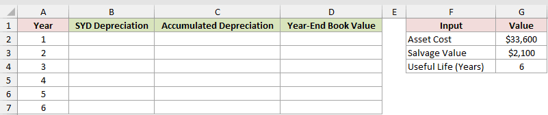
The first calculation returns all six annual depreciation amounts with one formula.
Here is the SYD formula:
=SYD(G2,G3,G4,A2:A7)
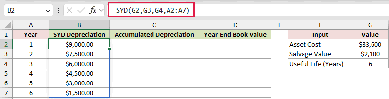
The period argument is the Year range A2:A7, so the formula spills six results into B2:B7.
Range-based SYD formulas spill in Excel 2021, Excel 2024, and Microsoft 365. Year 1 returns $9,000.00, and Year 6 returns $1,500.00.
Next, we want a running total of the depreciation recorded through each year.
Here is the accumulated depreciation formula entered in C2 and copied down through C7:
=SUM($B$2:B2)
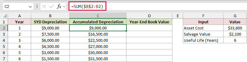
The first reference stays fixed at B2, while the second expands as the formula is copied down.
Each row sums the SYD column from B2 through its own row, giving a running total. This formula is copied down rather than spilled by design.
The accumulated amount reaches $31,500.00 in C7, which is the full difference between the asset’s cost and salvage value.
Finally, we want the year-end book value after each accumulated amount.
Here is the book value formula:
=G2-C2:C7
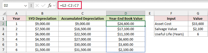
The formula subtracts every accumulated depreciation value from the original cost in G2. It spills the results into D2:D7.
Book value falls from $24,600.00 after Year 1 to $2,100.00 after Year 6. That final amount matches the salvage value.
SYD expense shrinks because the remaining-life digit drops each year. Year 1 takes 6/21 of the $31,500 depreciable base, compared with 1/6 under straight-line depreciation (SLN).
That makes SYD front-loaded, like the DB function, although the two methods calculate depreciation differently.
Example 3: Depreciate Several Assets at Once
Here’s a practical register with assets at different stages of their useful lives.
Below is a landscaping company’s asset list. Each row has its own cost, salvage value, useful life, and year in service. Column F will hold this year’s depreciation.
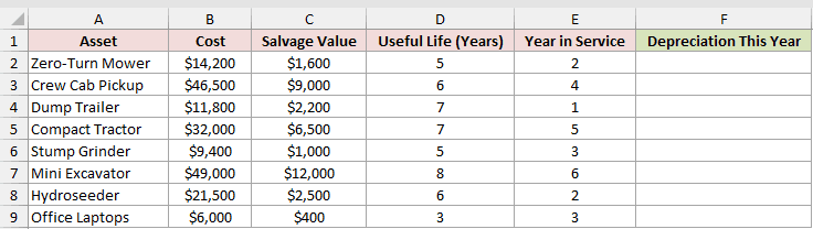
A single formula will calculate the current depreciation amount for every asset.
Here is the formula:
=SYD(B2:B9,C2:C9,D2:D9,E2:E9)
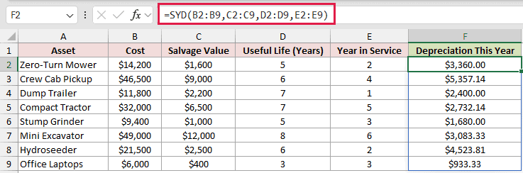
Each SYD argument uses a matching range, so Excel evaluates the values on the same row and spills eight results into F2:F9.
The zero-turn mower returns $3,360.00 in F2. The crew cab pickup returns $5,357.14, while the office laptops return $933.33.
This setup is handy at year-end because each asset can have a different cost, life, and current period.
Pro Tip: SYD returns #NUM! when a period is zero or greater than the asset’s useful life. Check fully depreciated assets before applying the function to a register.
Example 4: Find Book Value After Several Years
Sometimes you need the current book value without displaying a complete schedule.
Below is an input card for an $18,400 server with $1,600 salvage, a four-year life, and two years used. The final rows will hold the results.
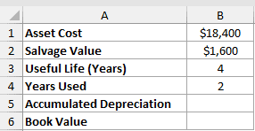
First, we’ll calculate the depreciation accumulated during the server’s first two years.
Here is the accumulated depreciation formula:
=SUM(SYD(B1,B2,B3,SEQUENCE(B4)))
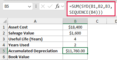
SEQUENCE creates the periods through the number of years in B4. SYD calculates each period, and SUM combines those amounts into one result.
The formula returns $11,760.00 in B5. SEQUENCE requires Excel 2021 or later.
We can now subtract accumulated depreciation from the original cost.
Here is the book value formula:
=B1-B5
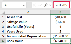
The result in B6 is $6,640.00. Change the years used in B4, and both result cells update for the new point in the asset’s life.
Example 5: Prorate SYD by Fiscal Year
The last example handles an asset placed in service partway through a fiscal year.
Below is a six-year fiscal schedule for a pickup truck. Inputs in E2:E5 hold its $52,000 cost, $7,000 salvage, five-year life, and four months in Year 1.
Column B will hold depreciation.
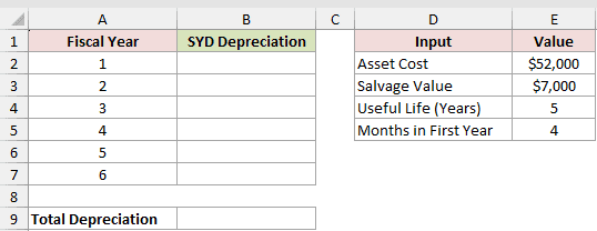
We want to spread each asset year’s depreciation across the fiscal years in which it falls.
Here is the prorated SYD formula:
=IF(A2:A7<=E4,SYD(E2,E3,E4,A2:A7),0)*E5/12+IF(A2:A7>1,SYD(E2,E3,E4,A2:A7-1),0)*(12-E5)/12
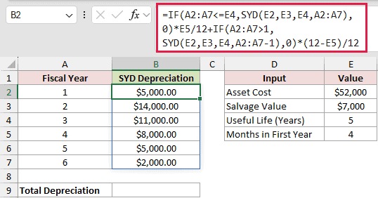
One formula entered in B2 spills six fiscal-year results through B7 in Excel 2021, Excel 2024, and Microsoft 365.
The first IF weights the current asset year’s depreciation by the four months held in E5.
The second IF brings in the previous asset year’s depreciation for the remaining eight months. Periods outside the useful life contribute zero.
This is why a five-year asset spans six fiscal years. The schedule returns $5,000.00 in the first fiscal year and $2,000.00 in the sixth.
We also want to confirm that the prorated schedule records all depreciation.
Here is the total formula:
=SUM(B2:B7)
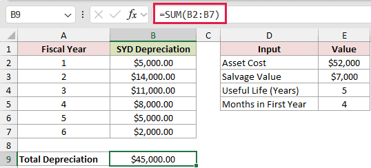
The total in B9 is $45,000.00. That matches the difference between the truck’s $52,000 cost and $7,000 salvage value, so proration has not lost any depreciation.
Pro Tip: SYD has no month argument. Dividing an annual amount by 12 gives monthly portions, while defining the useful life in months creates a different depreciation curve.
Tips & Common Mistakes
- A fractional per is accepted rather than rounded. It returns an interpolated amount that belongs to no single year, so check for accidental decimals.
- Excel 2019 and earlier need one formula per result cell.
- Keep the spill area empty. A blocked output range returns
#SPILL!, while an implicit-intersection@reduces a range formula to one result. - The sum of all valid periods should equal cost minus salvage. Use that check to catch an incomplete or incorrectly prorated schedule.
SYD works well when an asset should lose more book value early and less later.
The key is matching each SYD period to the reporting period in your depreciation records.
Related Excel Functions / Articles:
