
The CHISQ.DIST.RT function in Excel returns the right-tailed probability for a chi-square value and specified degrees of freedom.
When the value is a chi-square test statistic, that probability is the p-value. It measures how much of the distribution lies beyond the statistic.
In this article, I’ll show you how to build goodness-of-fit and independence tests, adjust degrees of freedom after estimating a parameter, and run an upper-tail variance test.
CHISQ.DIST.RT Function Syntax in Excel
The function needs a chi-square value and its degrees of freedom.
=CHISQ.DIST.RT(x,deg_freedom)
- x (required) is the nonnegative value at which you want the right-tailed probability.
- deg_freedom (required) is the degrees of freedom for the chi-square distribution. Excel truncates a non-integer value.
When to Use CHISQ.DIST.RT Function
- Convert an existing chi-square statistic and its degrees of freedom into a right-tailed p-value.
- Build a manual goodness-of-fit test and inspect which categories contribute most to the statistic.
- Run an independence test when you want to calculate and verify the degrees of freedom yourself.
- Adjust the degrees of freedom when a model parameter was estimated from the same data.
- Test whether observed variation is greater than a planned variance.
Example 1: Find P-Values From Reported Statistics
Let’s start with results that already include a chi-square statistic and degrees of freedom.
Below is the dataset. It lists each survey finding, its statistic, its degrees of freedom, and an empty p-value column for the results.
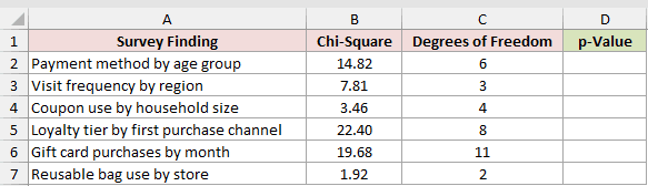
We want one formula to return the right-tailed p-value for every reported finding.
Here is the formula:
=CHISQ.DIST.RT(B2:B7,C2:C7)
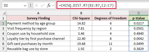
The formula pairs each statistic in column B with the degrees of freedom on the same row. The results spill down column D.
In Excel 2021, Excel 2024, and Microsoft 365, a range formula like this spills automatically. In Excel 2019 and earlier, enter a row formula and fill it down.
At a 0.05 cutoff, the visit-frequency result narrowly misses significance. Its statistic is 7.81 with 3 degrees of freedom, and its p-value is 0.0501.
The gift-card result narrowly makes the cutoff. Its statistic is 19.68 with 11 degrees of freedom, and its p-value is 0.0499.
That comparison also shows why a chi-square statistic is not meaningful by itself. You need the matching degrees of freedom before interpreting it.
Example 2: Build a Goodness-of-Fit Test
Now let’s test whether parking tickets follow the distribution of parking meters across several zones.
Below is the dataset. It contains meters and tickets by zone, empty expected and contribution columns, and a result card for the statistic, degrees of freedom, and p-value.

We first want to allocate the total tickets according to each zone’s share of all parking meters.
Here is the expected-ticket formula:
=SUM(C2:C6)*B2:B6/SUM(B2:B6)

The formula divides each zone’s meter count by the total meter count, applies that share to all tickets, and spills the expected counts down column D.
Now we’ll calculate each zone’s contribution to the chi-square statistic.
Here is the contribution formula:
=(C2:C6-D2:D6)^2/D2:D6

That one formula spills down column E. Each result squares the gap between observed and expected tickets, then divides by the expected count.
Larger values identify zones with larger departures.
Adding those contributions gives us the test statistic.
Here is the formula:
=SUM(E2:E6)

The chi-square statistic is 21.550. Riverfront contributes 14.003, so that zone accounts for most of the departure from the expected pattern.
The category count gives us the degrees of freedom.
Here is the formula:
=ROWS(C2:C6)-1

The result is 4 degrees of freedom.
We’ve got the statistic and degrees of freedom, so CHISQ.DIST.RT can return the p-value.
Here is the formula:
=CHISQ.DIST.RT(H2,H3)

The p-value is 0.0002. That is well below 0.05, so the ticket distribution differs from the meter distribution.
CHISQ.TEST can return the same p-value from the observed and expected ranges. It does not show the statistic or which zone drives it.
Example 3: Test Independence With Correct Degrees of Freedom
Here’s a two-way table that compares library genres with checkout formats.
Below is the dataset. It includes observed counts, SUM totals for the expected-count table, an empty expected table, and a result card for the test calculations.
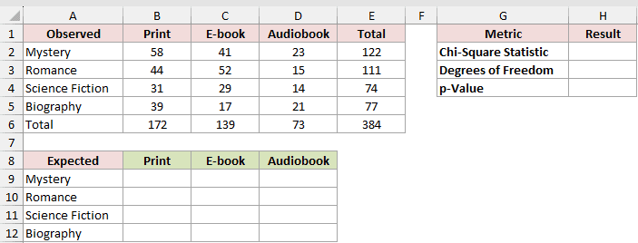
We first want the expected count for every genre and format if the two variables are independent.
Here is the formula:
=E2:E5*B6:D6/E6
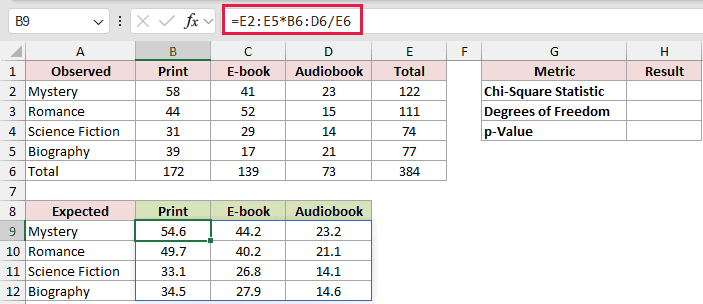
Excel combines each row total with every column total, then divides by the grand total. The formula spills into the complete expected table.
The expected table lets us compare all observed and expected cells for the chi-square statistic.
Here is the formula:
=SUM((B2:D5-B9:D12)^2/B9:D12)
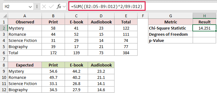
The result is a chi-square statistic of 14.251.
In Excel 2019 and earlier, use SUMPRODUCT with the same arguments for this array calculation.
The table’s row and column counts give us the degrees of freedom.
Here is the formula:
=(ROWS(B2:D5)-1)*(COLUMNS(B2:D5)-1)
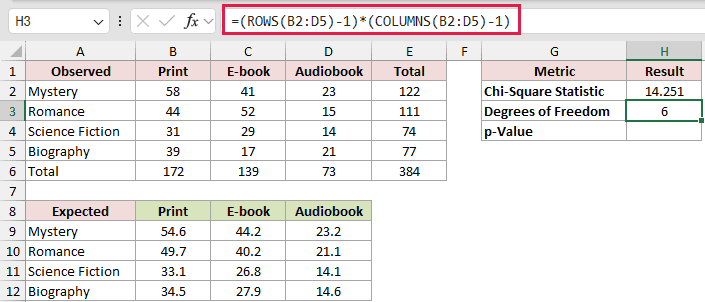
The table has 6 degrees of freedom. Counting all observed cells and subtracting one would be the wrong method.
We’ve got both inputs, so CHISQ.DIST.RT can return the right-tailed p-value.
Here is the formula:
=CHISQ.DIST.RT(H2,H3)
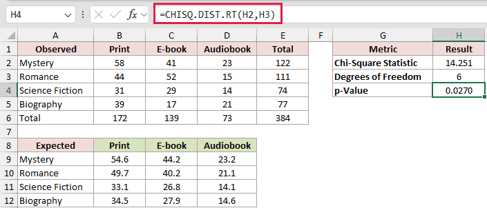
The correct p-value is 0.0270. Using the wrong degrees of freedom value of 11 returns 0.2194 and reverses the decision at a 0.05 cutoff.
Example 4: Adjust Degrees of Freedom for an Estimated Rate
This example checks whether seed germination counts follow a binomial pattern.
Below is the dataset. Each tray cell holds four seeds. Column A shows how many of the four germinated in a cell, from 0 to 4.
Column B shows how many tray cells had each germination count. Column C and the result card contain empty cells for the calculations.
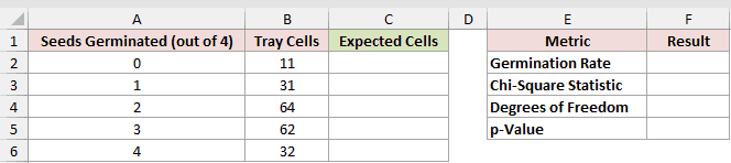
We first need to estimate the germination rate from the observed tray-cell counts.
Here is the formula:
=SUMPRODUCT(A2:A6,B2:B6)/(4*SUM(B2:B6))
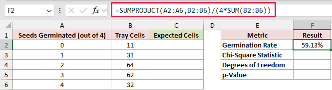
SUMPRODUCT calculates the total germinated seeds. The denominator is the total seeds planted: four seeds per cell times the number of cells.
The estimated germination rate is 59.13%.
We’ll use that rate to calculate the expected tray-cell counts.
Here is the formula:
=SUM(B2:B6)*BINOM.DIST(A2:A6,4,F2,FALSE)
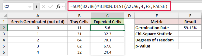
BINOM.DIST returns the expected share for each possible germination count. Multiplying by the total number of tray cells turns those shares into expected counts.
The 4 inside BINOM.DIST is the number of seeds in each cell. The single formula spills the expected counts down column C.
With the expected counts in place, we can calculate the chi-square statistic.
Here is the formula:
=SUM((B2:B6-C2:C6)^2/C2:C6)
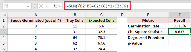
The chi-square statistic is 8.637.
Because the germination rate came from this dataset, it costs one additional degree of freedom.
Here is the adjusted formula:
=ROWS(B2:B6)-1-1
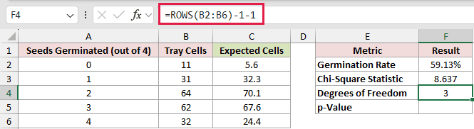
The adjusted result is 3 degrees of freedom.
We’ve adjusted the degrees of freedom, so CHISQ.DIST.RT can return the p-value.
Here is the formula:
=CHISQ.DIST.RT(F3,F4)
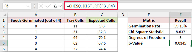
The p-value is 0.0345, which falls below 0.05.
Pro Tip: CHISQ.TEST would infer 4 degrees of freedom from the range shape and return 0.0708. That is the wrong comparison here because the germination rate was estimated from the same data.
Example 5: Run an Upper-Tail Variance Test
For the last example, we’ll check whether daily unit demand varies more than planned.
Below is the dataset. It contains dates and units sold, plus the planned standard deviation in the Input/Value card.
The Metric/Result card labels Sample SD, Chi-Square Statistic, Degrees of Freedom, and p-Value, with empty result cells ready for the formulas.
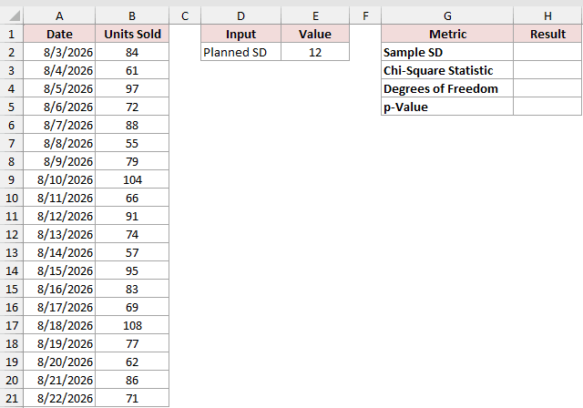
We first want the sample standard deviation of the daily unit counts.
Here is the formula:
=STDEV.S(B2:B21)
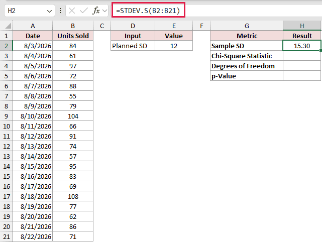
The sample standard deviation is 15.30, compared with the planned value of 12 in cell E2.
We can now build the chi-square statistic using the sample deviation in H2 and the planned deviation in E2.
Here is the formula:
=(COUNT(B2:B21)-1)*H2^2/E2^2
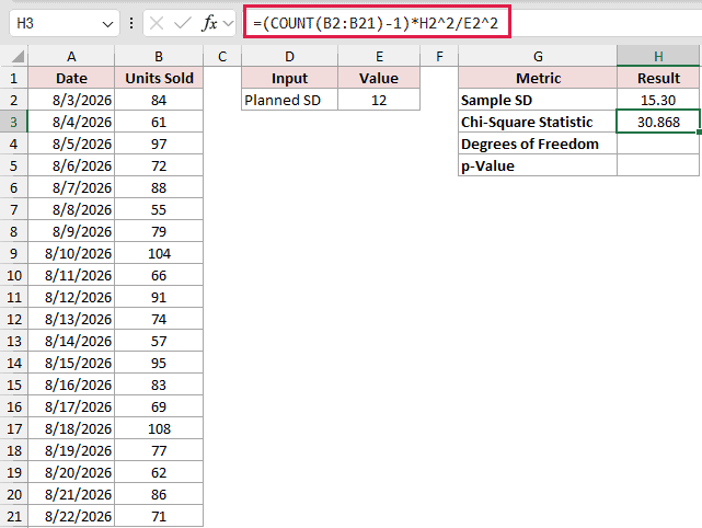
The statistic is 30.868.
The degrees of freedom equal the count of observations minus one.
Here is the formula:
=COUNT(B2:B21)-1
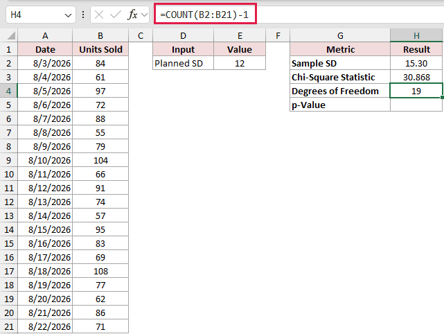
The result is 19 degrees of freedom.
That gives us both inputs for the right-tailed p-value.
Here is the formula:
=CHISQ.DIST.RT(H3,H4)
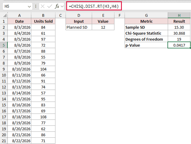
The p-value is 0.0417. At a 0.05 cutoff, the observed variation is greater than the planned variance.
Pro Tip: Reference H2 instead of typing its displayed 15.30. Typing that rounded value produces 30.887 instead of the workbook’s full-precision result of 30.868.
Tips & Common Mistakes
- CHISQ.DIST.RT is available in Excel 2010 and later.
- Both arguments are required. A negative x value or degrees of freedom below 1 returns #NUM!.
- Excel truncates decimal degrees of freedom. Make sure the value represents the test you actually performed before using it.
- An x value of 0 returns 1. A blank x cell also returns 1, so validate missing inputs before interpreting the result.
- CHIDIST is the legacy function and returns the same right-tailed value.
CHISQ.DISTreturns the left-tail probability whencumulativeis TRUE. For example,1-CHISQ.DIST(3,4,TRUE)equalsCHISQ.DIST.RT(3,4), or 0.557825.CHISQ.INV.RTreturns the chi-square value for a given right-tail probability. When you feed it alpha, that value is the critical value. - CHISQ.TEST returns a p-value from observed and expected ranges. Use CHISQ.DIST.RT when you already have the statistic or need to control the degrees of freedom.
- Very small p-values can look rounded away in a fixed-decimal format. Switch to scientific notation before reporting the value as zero.
- A blocked spill range returns #SPILL!. Clear the output cells so Excel can place every result.
- A p-value above your cutoff does not prove that the data fits perfectly. It means the test did not find enough evidence against the expected pattern.
CHISQ.DIST.RT keeps the statistic and degrees of freedom in view, which makes unusual test setups easier to check.
Keep full-precision inputs in cells and reference them in later formulas. That matters most when a result sits close to a decision cutoff.
Other Excel articles you may also like:
