
The CHISQ.INV.RT function in Excel returns the chi-square value whose right-tail probability matches the probability you provide.
Give it a significance level to get a critical value. If you already have a p-value, it recovers the corresponding chi-square statistic without returning the p-value itself.
In this article, I’ll show you how to build a critical-value table, recover a statistic after chi-square tests, and test whether a process is too variable.
CHISQ.INV.RT Function Syntax in Excel
The function takes a right-tail probability and the required degrees of freedom.
=CHISQ.INV.RT(probability, deg_freedom)
- probability (required) is the right-tail probability associated with the chi-square value.
- deg_freedom (required) is the number of degrees of freedom for the distribution.
When to Use CHISQ.INV.RT Function
- Find the critical value for a right-tailed chi-square test.
- Build a table of critical values for several significance levels and degrees of freedom.
- Compare a calculated chi-square statistic with its cutoff.
- Recover a chi-square statistic when CHISQ.TEST has returned only a p-value.
- Test whether a process variance is higher than a target variance.
Example 1: Build a Chi-Square Critical-Value Table
Let’s start with a reusable table of right-tail critical values.
Below is a grid with degrees of freedom in column A, probability inputs across row 1, and an empty body ready for the critical values.
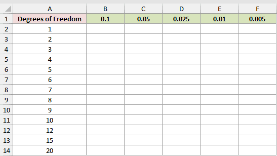
We want one formula to return every row and column intersection in the grid.
Here is the formula:
=CHISQ.INV.RT(B1:F1,A2:A14)
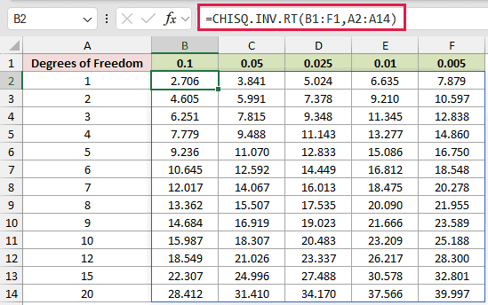
The formula in B2 pairs every probability in B1:F1 with every degree of freedom in A2:A14, then spills the full 13×5 table through B2:F14.
For 4 degrees of freedom, the 0.05 cutoff is 9.488. Reducing the probability to 0.005 raises the cutoff to 14.860.
This range formula spills in Excel 2021, Excel 2024, and Microsoft 365. In Excel 2019 and earlier, use mixed references and fill across and down.
Pro Tip: Keep the spill area empty. Any value blocking the output range makes Excel return #SPILL! instead of the critical-value table.
Example 2: Test Gym Check-In Patterns
Now let’s use a critical value to make a goodness-of-fit decision.
Below is the dataset with time slots, scheduled classes, check-ins, expected counts, and a 0.05 significance-level input in G1. The result card holds the test outputs.
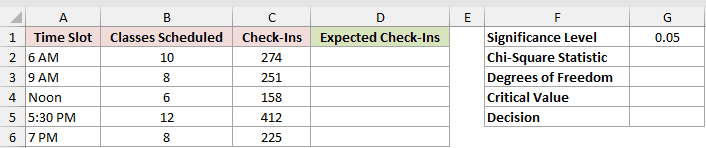
We want to check whether check-ins follow the pattern implied by the class schedule.
First, enter one formula in D2 to spill the five expected check-ins through D2:D6:
=SUM(C2:C6)*B2:B6/SUM(B2:B6)
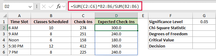
The formula allocates total check-ins according to each slot’s share of scheduled classes. The expected counts are 300.0, 240.0, 180.0, 360.0, and 240.0.
Next, calculate the chi-square statistic:
=SUM((C2:C6-D2:D6)^2/D2:D6)
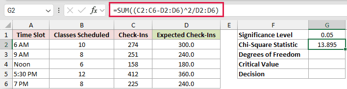
This adds each squared observed-minus-expected difference after dividing by its expected count. The statistic is 13.895.
In Excel 2019 and earlier, calculate the same statistic with SUMPRODUCT instead of the array-arithmetic SUM formula.
Now calculate the degrees of freedom:
=ROWS(C2:C6)-1
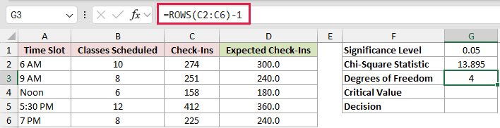
Goodness-of-fit degrees of freedom equal the category count minus 1. The formula returns 4.
Use the significance level and degrees of freedom to find the critical value:
=CHISQ.INV.RT(G1,G3)
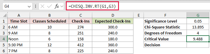
The critical value is 9.488. A statistic above this cutoff falls inside the rejection region.
Finally, return a clear decision:
=IF(G2>G4,"Significant","Not significant")
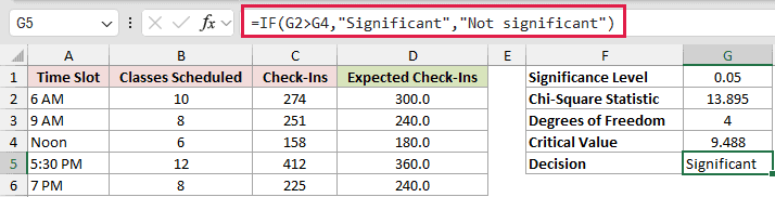
Because 13.895 is above 9.488, Excel returns Significant. The 5:30 PM slot has 412 check-ins against 360.0 expected. That is the largest gap.
CHISQ.DIST.RT returns the corresponding right-tail p-value of 0.0076, which reaches the same decision at the 0.05 significance level.
Pro Tip: The 13.895 statistic beats the 1% cutoff of 13.277 but not the 0.5% cutoff of 14.860.
Example 3: Recover a Statistic From a P-Value
Here’s a useful reporting trick when CHISQ.TEST has returned only a p-value.
Below is an observed station-by-rider table with SUM row and column totals, plus a significance-level input of 0.05 in G1.
The sheet also includes an expected-count table and a result card for the p-value, degrees of freedom, statistic, and cutoff.
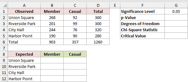
We want to recover the chi-square statistic and compare it with the critical value.
First, enter one formula in B9 to spill the full expected table through B9:C12. Nothing needs to be copied or filled:
=D2:D5*B6:C6/D6
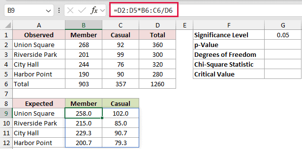
The formula multiplies each row total by each column total, then divides by the grand total. The smallest displayed expected count is 79.3.
Now return the p-value from the observed and expected ranges:
=CHISQ.TEST(B2:C5,B9:C12)
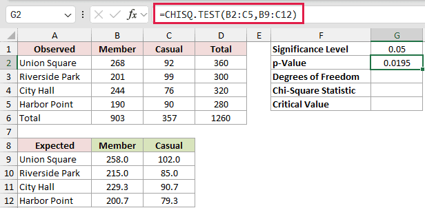
CHISQ.TEST returns 0.0195. It does not return the chi-square statistic needed for a detailed report.
Calculate the degrees of freedom from the observed table’s shape:
=(ROWS(B2:C5)-1)*(COLUMNS(B2:C5)-1)
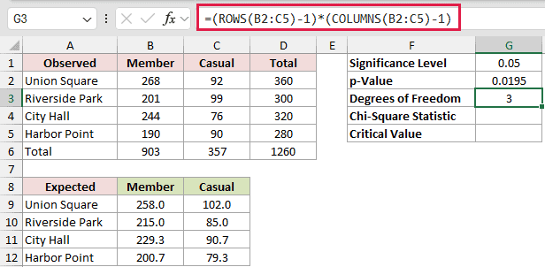
An independence test uses rows minus 1 multiplied by columns minus 1. The formula returns 3.
Feed the p-value into CHISQ.INV.RT to recover the statistic:
=CHISQ.INV.RT(G2,G3)
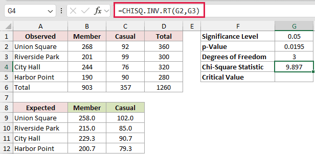
The recovered chi-square statistic is 9.897. This is the inverse operation behind the right-tail p-value.
Then calculate the critical value from the significance level:
=CHISQ.INV.RT(G1,G3)
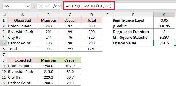
The critical value is 7.815. The statistic is above the cutoff, while 0.0195 is below 0.05, so both routes reach the same conclusion.
Example 4: Check Several Chi-Square Tests
Now let’s check a log containing several survey tests at once.
Below is the dataset with each crosstab’s row count, column count, and statistic, plus columns waiting for degrees of freedom, critical values, and decisions.
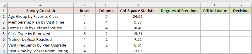
We want every test to use the cutoff that matches its own table shape.
First, calculate each test’s degrees of freedom:
=(B2:B8-1)*(C2:C8-1)
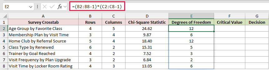
The formula applies the independence-test rule to each row and spills the results down column E.
Next, return the matching critical value for every test:
=CHISQ.INV.RT(0.05,E2:E8)
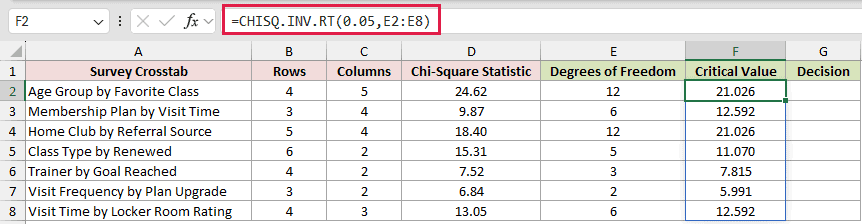
Each row gets its own cutoff. The values range from 5.991 to 21.026 because the degrees of freedom differ.
Now compare every statistic with its matching cutoff:
=IF(D2:D8>F2:F8,"Significant","Not significant")
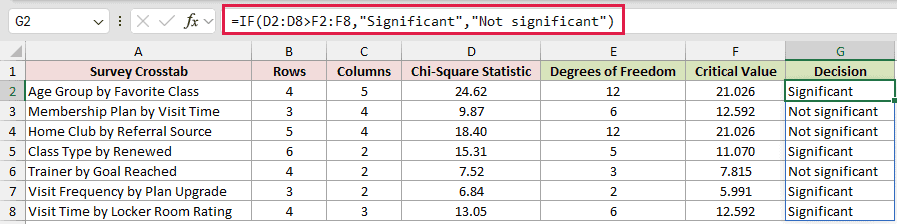
A larger statistic does not automatically mean a stronger result. The 18.40 statistic is below its 21.026 cutoff, while 15.31 is above 11.070.
The closest call is 7.52 against 7.815. Excel correctly labels that test Not significant.
Example 5: Run a Right-Tailed Variance Test
Finally, let’s test whether espresso extraction times vary more than the target allows.
Below are 15 extraction times, a target standard deviation, a significance-level input, and a result card for sample size, sample deviation, statistic, cutoff, and decision.
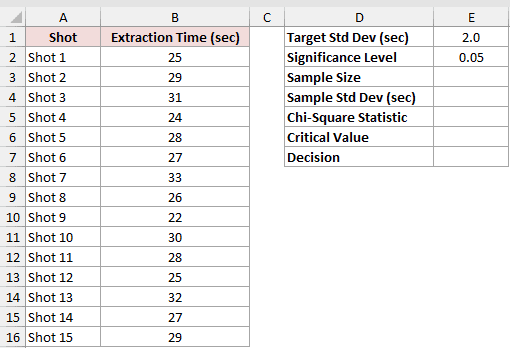
We want to test whether the process variance is higher than the target variance.
First, count the extraction times:
=COUNT(B2:B16)
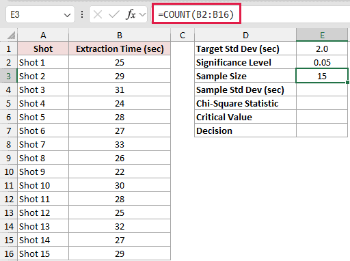
The COUNT formula returns a sample size of 15.
Next, calculate the sample standard deviation:
=STDEV.S(B2:B16)
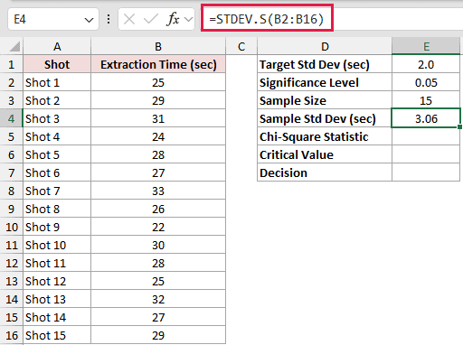
The sample standard deviation is 3.06 seconds, compared with the 2.0-second target in E1.
Now calculate the chi-square statistic:
=(E3-1)*E4^2/E1^2
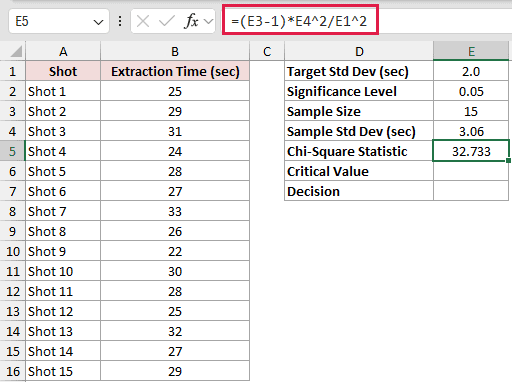
The formula compares sample variance with target variance and scales it by the degrees of freedom. The statistic is 32.733.
Use the right-tail inverse to find the critical value:
=CHISQ.INV.RT(E2,E3-1)
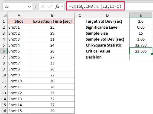
The critical value is 23.685. The sample statistic must exceed this cutoff to show greater variability.
Finally, return the test decision:
=IF(E5>E6,"More variable than target","Within target")
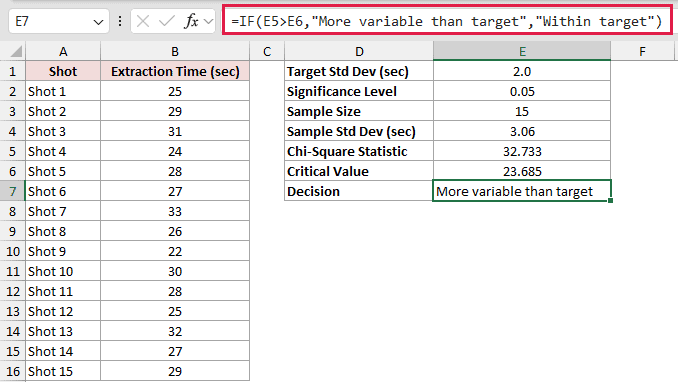
Because 32.733 exceeds 23.685, Excel returns More variable than target.
This chi-square variance test assumes the sampled measurements come from a normally distributed population.
Tips & Common Mistakes
- CHISQ.INV.RT returns a cutoff when probability is an alpha value and a statistic when probability is a p-value. It never returns the p-value itself.
- Goodness-of-fit and independence tests are right-tailed. Pass the full significance level, not half of it.
- Do not swap CHISQ.INV.RT for CHISQ.INV. At probability 0.05 and 4 degrees of freedom, they return 9.487729 and 0.710723 because they use opposite tails.
- Probability 1 returns 0, while probability 0 or a blank probability returns #NUM!.
- Excel truncates decimal degrees of freedom. Use the correct whole-number rule for your test instead of relying on that truncation.
- CHIINV is the legacy equivalent and returns the same right-tail value. CHISQ.INV.RT has been available since Excel 2010.
- Numeric text such as
"0.05"is converted, while nonnumeric text returns #VALUE!. - An
@before a range-based formula collapses it to one value. A blocked spill range returns #SPILL!.
Treat the probability as the right-tail area you already know. The returned chi-square value becomes the cutoff or recovered statistic you need for the next decision.
Related Excel Functions / Articles:
