
Excel’s CHISQ.INV function returns the chi-square value whose left-tail area equals the given probability, for the given degrees of freedom.
That cutoff helps you decide whether observed variation is unusually low or place bounds around a variance estimate.
Tail direction matters here. CHISQ.INV works from the left, while CHISQ.INV.RT and the legacy CHIINV function work from the right.
In this article, I’ll show you how to calculate lower cutoffs, build standard-deviation limits, and replace old CHIINV formulas without changing their meaning.
CHISQ.INV Function Syntax in Excel
The CHISQ.INV function uses a probability and degrees of freedom to return a left-tail chi-square cutoff.
=CHISQ.INV(probability, deg_freedom)
- probability (required) is the left-tail cumulative probability associated with the cutoff.
- deg_freedom (required) is the number of degrees of freedom for the distribution.
When to Use CHISQ.INV Function
- Find a lower critical value for a left-tailed chi-square test.
- Test whether a process has become less variable.
- Build confidence intervals for a population variance or standard deviation.
- Set lower and upper variability limits for quality-control checks.
- Convert a right-tail probability before replacing a legacy CHIINV formula.
Example 1: Find Lower Chi-Square Critical Values
Let’s start with several instrument validation plans.
Below is the dataset. It lists each instrument, its replicate readings, its significance level, and an empty column for the lower critical value.
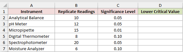
We want one formula to calculate every plan’s left-tail cutoff.
Here is the formula:
=CHISQ.INV(C2:C7,B2:B7-1)
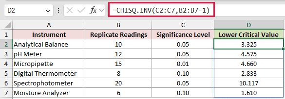
The formula uses each significance level as the left-tail probability. It subtracts one from each replicate count to get degrees of freedom.
The Analytical Balance returns 3.325, while the Spectrophotometer returns 10.117.
CHISQ.INV is available in Excel 2010 and later. This range formula spills in Excel 2021, Excel 2024, and Microsoft 365.
In Excel 2019 and earlier, calculate the rows individually and fill the formula down.
Pro Tip: For a one-sample variance calculation, degrees of freedom are the sample size minus one. Using the full sample size changes the cutoff.
Example 2: Test for Lower Process Variation
Now let’s test whether delivery times became more consistent after a routing change.
Below is the dataset. It contains delivery IDs and times, plus Old System Std Dev (min) 8 and Significance Level 0.05 as inputs.
Labeled cells hold the sample calculations, cutoff, and decision.
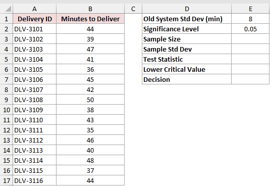
We want to compare the delivery-time statistic with a lower critical value.
First, COUNT finds the sample size:
=COUNT(B2:B17)
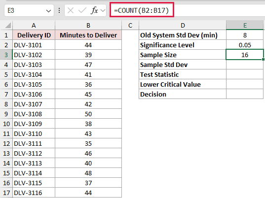
Cell E3 returns 16.
Next, STDEV.S calculates the sample standard deviation:
=STDEV.S(B2:B17)
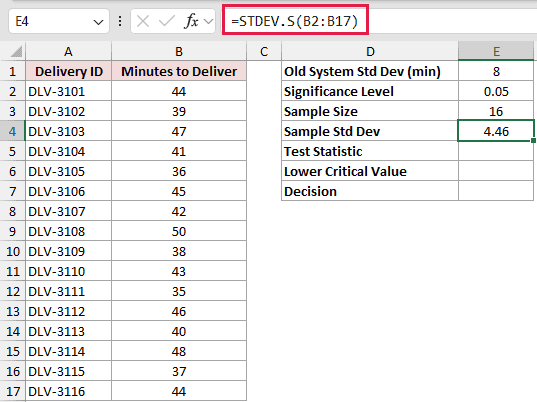
Cell E4 returns 4.46.
The test statistic uses the sample result and the old system’s standard deviation:
=(E3-1)*E4^2/E1^2
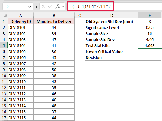
Cell E5 returns 4.663.
CHISQ.INV calculates the lower critical value:
=CHISQ.INV(E2,E3-1)
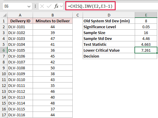
Cell E6 returns 7.261.
Finally, IF compares the statistic with that cutoff:
=IF(E5<E6,"Less variable","Not proven")
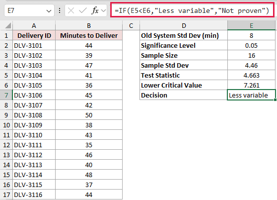
The statistic is below the lower cutoff, so cell E7 returns “Less variable”.
The left-tail probability from CHISQ.DIST is =CHISQ.DIST(E5,E3-1,TRUE), which returns 0.005385 and supports the same decision.
Example 3: Build a Variance Confidence Interval
Here’s a more detailed use of CHISQ.INV with tablet weights.
Below is the dataset. It lists tablet weights and a confidence-level input, plus labeled cells for the sample measures, chi-square values, and interval limits.
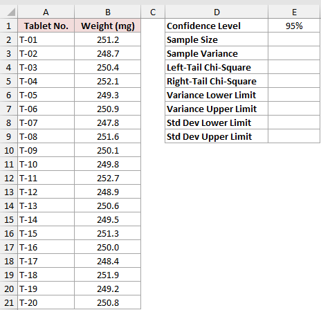
We want confidence limits for both the variance and standard deviation.
COUNT finds the sample size:
=COUNT(B2:B21)
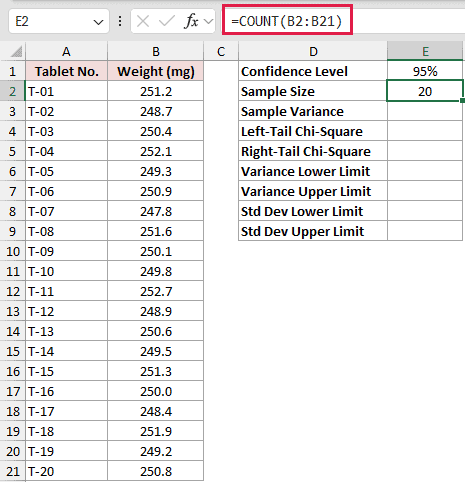
Cell E2 returns 20.
VAR.S calculates the sample variance:
=VAR.S(B2:B21)
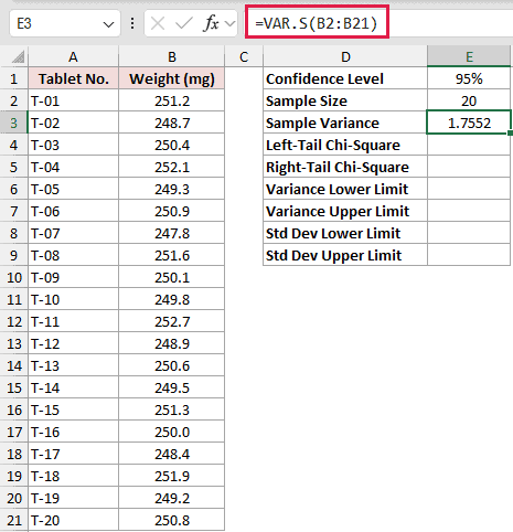
Cell E3 returns 1.7552.
CHISQ.INV returns the left-tail chi-square value:
=CHISQ.INV((1-E1)/2,E2-1)
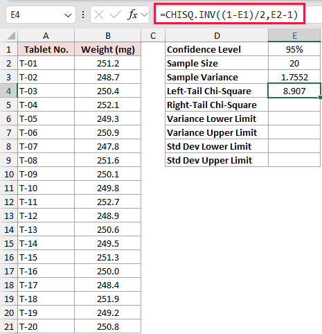
Cell E4 returns 8.907.
CHISQ.INV.RT returns the matching right-tail value:
=CHISQ.INV.RT((1-E1)/2,E2-1)
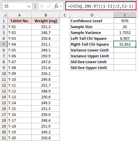
Cell E5 returns 32.852.
The right-tail value divides into the lower variance limit:
=(E2-1)*E3/E5
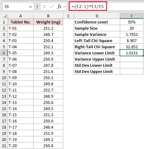
Cell E6 returns 1.0151.
The left-tail value divides into the upper variance limit:
=(E2-1)*E3/E4
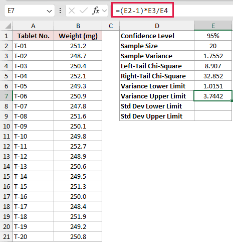
Cell E7 returns 3.7442. The variance interval is not symmetric around the sample variance.
Take the square root of the lower variance limit to convert it to a standard-deviation limit:
=SQRT(E6)
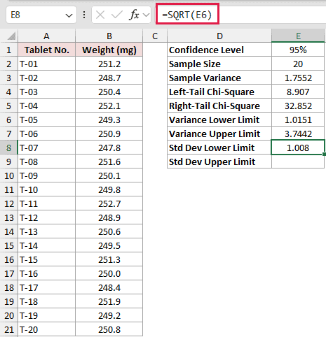
Cell E8 returns 1.008.
Do the same for the upper variance limit:
=SQRT(E7)
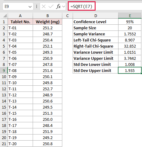
Cell E9 returns 1.935. These standard-deviation limits use the same confidence level as the variance interval.
Pro Tip: The smaller left-tail chi-square value belongs in the denominator of the upper variance limit. Swapping the two cutoffs reverses the interval.
Example 4: Set Two-Sided Standard Deviation Limits
Next, we’ll flag daily sensor readings that look too steady or too noisy.
Below is the dataset. It contains dates, daily sample standard deviations, and an empty status column.
The settings card has Sensor Std Dev (°F) 0.4, Readings per Day 8, Significance Level 0.01, and four empty labeled cells.
Those cells are Lower Chi-Square Cutoff, Upper Chi-Square Cutoff, Lowest OK Std Dev, and Highest OK Std Dev.
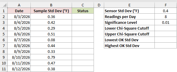
We want lower and upper standard-deviation limits, followed by a status for every day.
The lower cutoff uses half the significance level:
=CHISQ.INV(F3/2,F2-1)
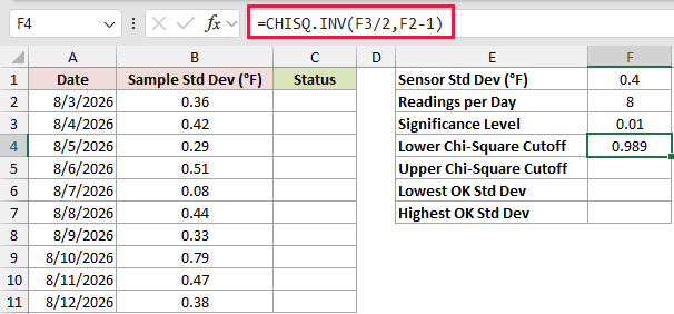
Cell F4 returns 0.989.
The upper cutoff uses the probability from the other tail:
=CHISQ.INV(1-F3/2,F2-1)
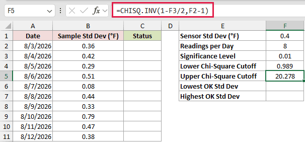
Cell F5 returns 20.278. Splitting the significance level across both tails also catches unusually low variation.
The first rescaling formula returns the lowest acceptable standard deviation:
=F1*SQRT(F4/(F2-1))
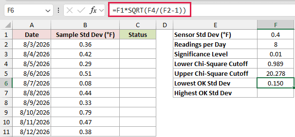
Cell F6 returns 0.150.
The second rescaling formula returns the highest acceptable standard deviation:
=F1*SQRT(F5/(F2-1))
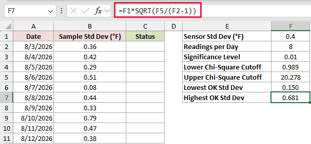
Cell F7 returns 0.681.
The status formula compares every daily value with those limits:
=IF(B2:B11<F6,"Too steady",IF(B2:B11>F7,"Too noisy","OK"))
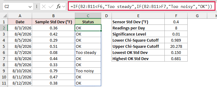
The formula spills down column C. The 8/7/2026 reading of 0.08 returns “Too steady”, while 8/10/2026 at 0.79 returns “Too noisy”.
A very low standard deviation can signal a stuck sensor, so it deserves attention alongside excessive noise.
Example 5: Replace Legacy CHIINV Correctly
Finally, let’s fix an easy migration mistake in older workbooks.
Below is the dataset. It lists old reports, right-tail probabilities, and degrees of freedom, with two comparison columns and a final column for the straight-renaming mistake.

We want to preserve each old CHIINV result when updating the formulas.
Here is the legacy CHIINV formula:
=CHIINV(B2:B6,C2:C6)

Column D returns the old right-tail cutoffs, including 9.488 for Store Foot Traffic and 11.345 for Menu Item Mix.
CHISQ.INV can match those results after converting each probability to its left-tail equivalent:
=CHISQ.INV(1-B2:B6,C2:C6)

Column E matches column D. It returns 9.488 and 11.345 for those same reports.
Here is the straight-renaming mistake. Do not use it:
=CHISQ.INV(B2:B6,C2:C6)

The mistake treats a right-tail probability as a left-tail probability. It returns 0.711 instead of 9.488 for Store Foot Traffic.
For Shift Coverage, the same mistake returns 2.204 instead of 10.645. The direct replacement for CHIINV is CHISQ.INV.RT, not CHISQ.INV.
Pro Tip: Never replace CHIINV by changing only the function name to CHISQ.INV. Either use CHISQ.INV.RT or convert the probability to its left-tail equivalent.
Tips & Common Mistakes
- CHISQ.INV returns a cutoff, not a p-value. Use CHISQ.DIST, CHISQ.DIST.RT, or CHISQ.TEST when you need a probability.
- A probability of 0 returns 0. A probability of 1 returns #NUM!, while a blank probability cell quietly acts as 0.
- Degrees of freedom below 1 return #NUM!. Decimal values are truncated, so 2.3 behaves like 2.
- Numeric text such as
"0.05"converts successfully. Non-numeric text such asabcreturns #VALUE!. - Keep the spill area empty. Occupied output cells cause #SPILL!, while an implicit-intersection
@reduces the range calculation to one result. - A round trip through CHISQ.DIST recovers the original left-tail probability.
=CHISQ.DIST(CHISQ.INV(0.3,5),5,TRUE)returns 0.3. =CHISQ.INV(0.93,1)returns 3.283020.
CHISQ.INV is the direct choice when you need a left-tail chi-square cutoff.
For one-sample variance work, use n-1 degrees of freedom before trusting the cutoff.
Related Excel Functions / Articles:
