
Excel’s DVAR function returns the sample variance of numbers in a database field after applying criteria. It reduces all matching records to one value.
DVAR returns variance in squared units. Example 5 compares two groups’ spread as a ratio, while the square root returns the result to the field’s original scale.
In this article, I’ll show you how to build AND and OR criteria, interpret squared-unit results, and handle samples that are too small.
DVAR Function Syntax in Excel
The DVAR function needs a headed database, the field to measure, and a criteria range.
=DVAR(database, field, criteria)
- database (required) is the complete list, including its header row.
- field (required) identifies the column to measure by its quoted header, cell reference, or one-based column position.
- criteria (required) is a separate range containing at least one matching database header and a condition below it.
When to Use DVAR Function
- Estimate sample variance for records that meet one or more conditions.
- Compare how widely values vary across stores, departments, regions, or other groups.
- Apply AND or OR logic through a worksheet criteria range.
- Calculate conditional sample variance when Excel’s regular variance functions cannot accept criteria directly.
Example 1: Calculate Variance for One Store
Let’s start with one store selected from a sample of weekly records.
Below is the dataset. It lists week ending dates, stores, transactions, and weekly sales, with criteria for Maple Grove and two labelled result cells.
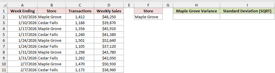
We want the sample variance for Maple Grove and its standard deviation on the original dollar scale.
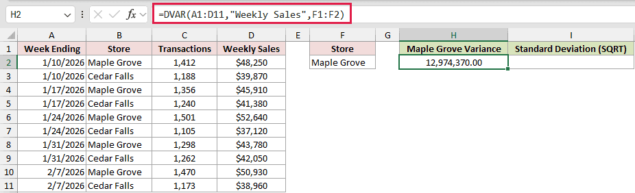
Here is the DVAR formula:
=DVAR(A1:D11,"Weekly Sales",F1:F2)
Here is the SQRT formula for the corresponding standard deviation:
=SQRT(H2)
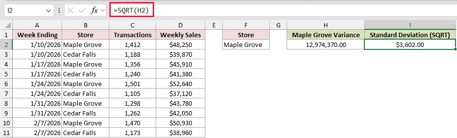
DVAR returns 12,974,370.00 in H2. The result measures the sales variance in squared dollars.
SQRT returns $3,602.00 in I2, putting the spread back on the original dollar scale. It equals DSTDEV under the same criteria.
Example 2: Apply Two AND Criteria
Now let’s narrow a sample with two conditions at once.
Below is the dataset. It contains store, region, format, and weekly sales columns, plus criteria for South supercenters and a labelled variance cell.
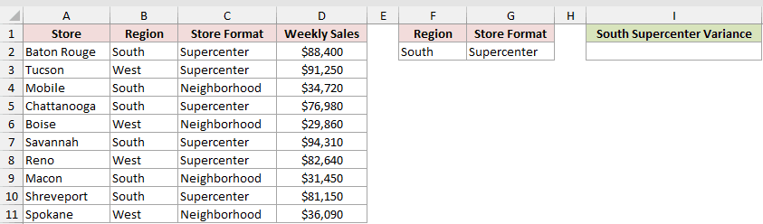
We want the sample variance of weekly sales for stores that meet both criteria.
Here is the formula:
=DVAR(A1:D11,"Weekly Sales",F1:G2)
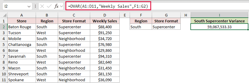
The result is 59,067,533.33. Both conditions sit on the same criteria row, so a record must be in the South and be a Supercenter.
Example 3: Combine OR Criteria
Here’s how to include either of two departments in the same calculation.
Below is the dataset. It lists week ending dates, departments, and weekly sales, with two department criteria and a labelled result cell.
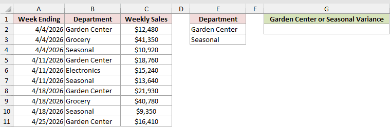
We want the sample variance for records from Garden Center or Seasonal.
Here is the formula:
=DVAR(A1:C11,3,E1:E3)
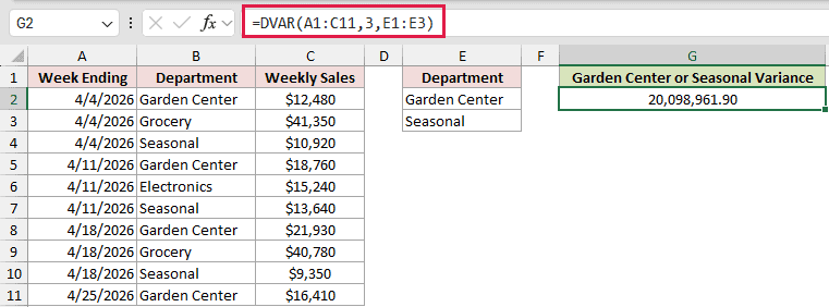
The result is 20,098,961.90. Conditions on separate criteria rows use OR logic, so either department can qualify.
The field argument is 3, which points to the third database column. A quoted header is safer if someone may insert or move columns later.
Pro Tip: Plain text criteria carry an implied wildcard at the end, so Garden Center also matches Garden Center Kiosk. Use ="=Garden Center" for an exact match.
Example 4: Exclude Closed Weeks
This example shows how one closure can distort a variance.
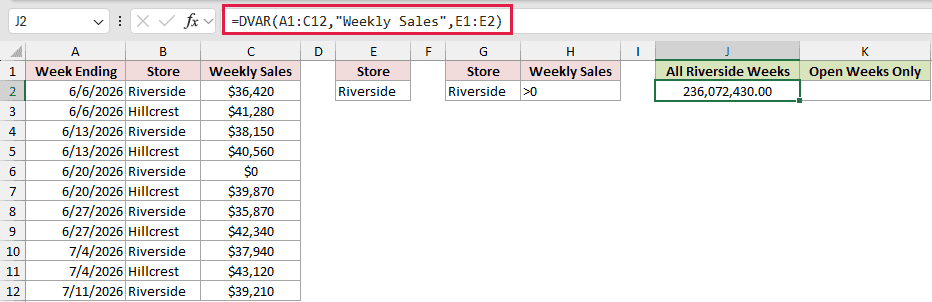
Below is the dataset. It lists week ending dates, stores, and weekly sales, plus two criteria blocks and labelled cells for All Riverside Weeks and Open Weeks Only.
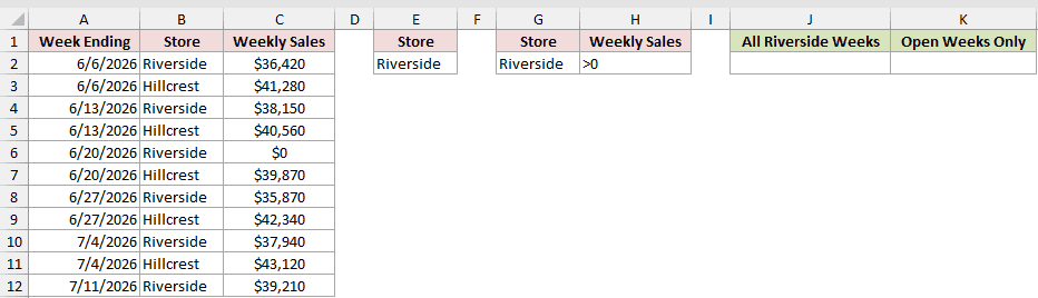
We want to compare the misleading all-weeks variance with a corrected calculation that excludes closed weeks.
Here is the misleading formula that includes every Riverside week:
=DVAR(A1:C12,"Weekly Sales",E1:E2)
Here is the corrected formula for open weeks only:
=DVAR(A1:C12,"Weekly Sales",G1:H2)
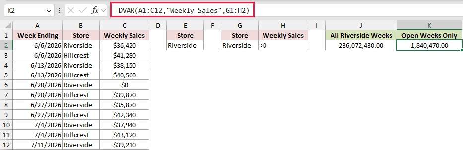
The first result, 236,072,430.00, is misleading because it treats the $0 storm-closure week as normal sales activity.
The corrected result is 1,840,470.00. The >0 condition keeps Riverside records while excluding the closed week.
Example 5: Compare Variance Between Groups
This example compares the spread of weekly sales at malls and strip centers.
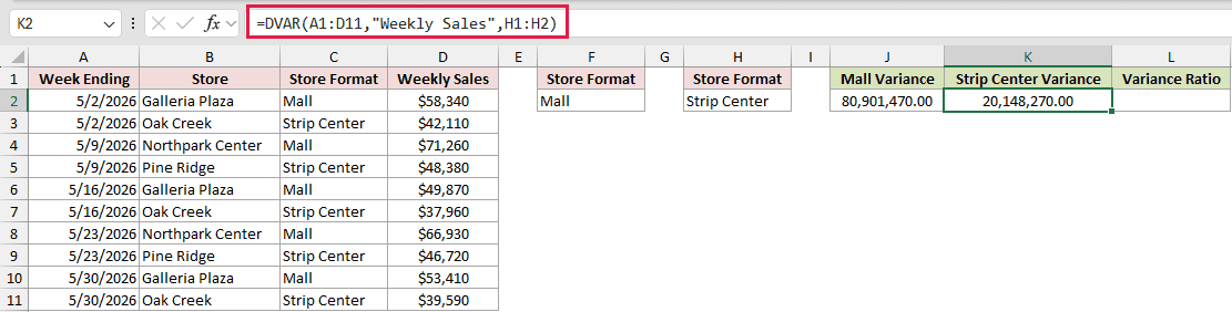
Below is the dataset. It lists sampled weeks, stores, formats, and weekly sales, with criteria plus labelled Mall Variance, Strip Center Variance, and Variance Ratio cells.
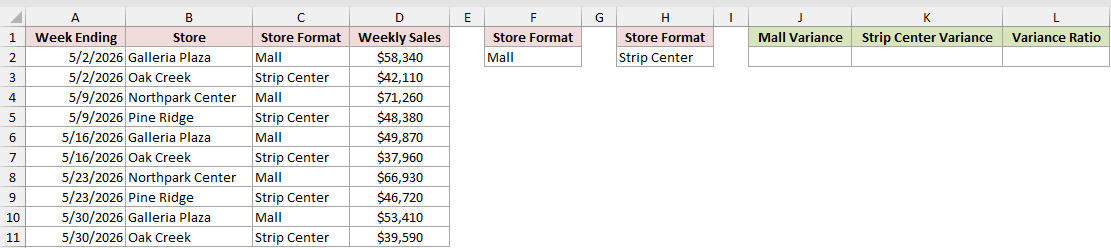
We want each format’s sample variance, followed by the ratio between them.
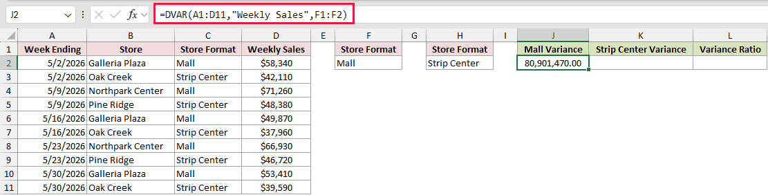
Here is the mall variance formula:
=DVAR(A1:D11,"Weekly Sales",F1:F2)
Here is the strip center variance formula:
=DVAR(A1:D11,"Weekly Sales",H1:H2)
Finally, divide the two variances:
=J2/K2
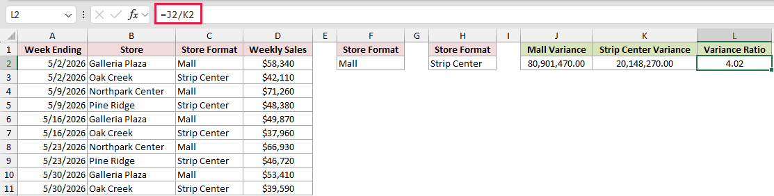
The mall variance is 80,901,470.00, while the strip center variance is 20,148,270.00. Their variance ratio is 4.02.
Because standard deviation is the square root of variance, that ratio means mall sales have roughly twice the standard-deviation spread.
Example 6: Compare DVAR With DVARP
The choice between sample and population variance depends on what the matching records represent.
Below is the dataset. It lists stores from two districts and their average weekly sales, with District 4 criteria and two labelled variance cells.
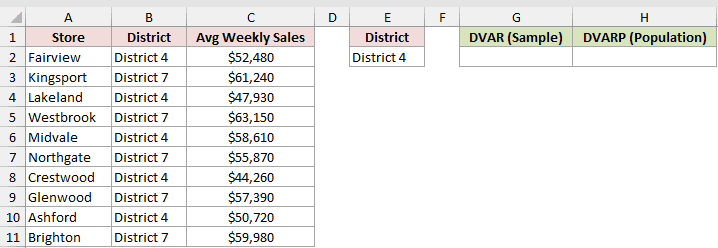
We want to compare DVAR’s sample calculation with DVARP for the complete group of five District 4 stores.
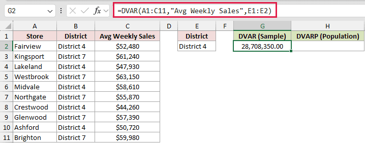
Here is the DVAR formula:
=DVAR(A1:C11,"Avg Weekly Sales",E1:E2)
And here is the DVARP comparison:
=DVARP(A1:C11,"Avg Weekly Sales",E1:E2)
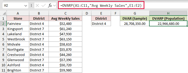
DVAR returns 28,708,350.00, but it treats the matched stores as a sample from a wider population.
DVARP returns 22,966,680.00. It’s the right fit because those five stores make up the whole group being described.
Example 7: Compare DVAR With VAR.S and FILTER
In Excel 2021 and later, you can use a formula-only route when your conditions already sit inside the formula.
Below is the dataset. It lists sampled weeks, fulfillment channels, and weekly sales, with Curbside Pickup criteria and labelled cells for both methods.
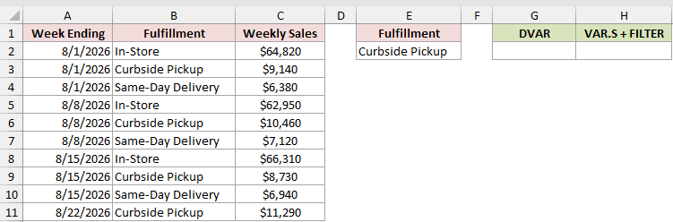
We want to compare DVAR with the modern conditional-variance route, because Excel has no VARIFS function.
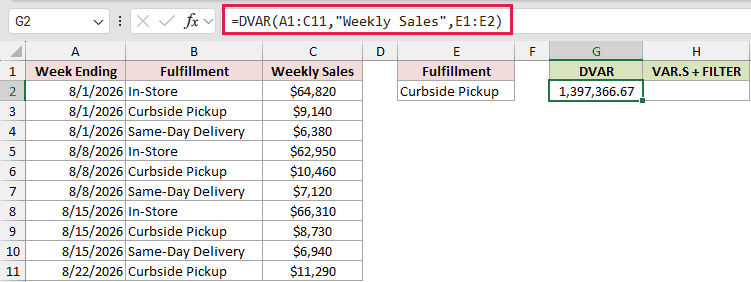
Here is the DVAR formula:
=DVAR(A1:C11,"Weekly Sales",E1:E2)
Here is the VAR.S and FILTER comparison:
=VAR.S(FILTER(C2:C11,B2:B11=E2))
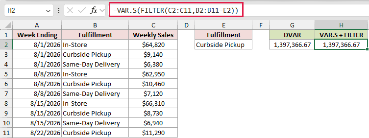
Both formulas return 1,397,366.67. DVAR reads a worksheet criteria block, while FILTER builds the qualifying array inside the formula.
FILTER works in Excel 2021, Excel 2024, and Microsoft 365. DVAR works in every current version of Excel.
Example 8: Guard Against One Match
A sample variance needs enough matching records to estimate spread.
Below is the dataset. It lists sampled weeks, stores, and weekly sales, with Lakewood criteria plus cells for the raw DVAR result and a guarded message.
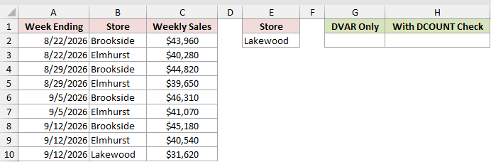
We want to show the deliberate error from one matching week, then replace it with a readable check.
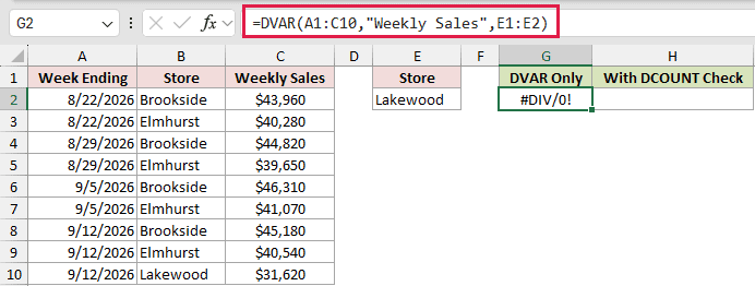
Here is the unguarded DVAR formula:
=DVAR(A1:C10,"Weekly Sales",E1:E2)
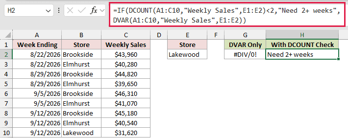
Here is the guarded formula:
=IF(DCOUNT(A1:C10,"Weekly Sales",E1:E2)<2,"Need 2+ weeks",DVAR(A1:C10,"Weekly Sales",E1:E2))
The raw DVAR cell deliberately returns #DIV/0! because Lakewood has one matching week and sample variance divides by n minus 1.
The guarded cell returns “Need 2+ weeks”. DCOUNT checks the number of matching numeric sales records before DVAR runs.
Tips & Common Mistakes
- Keep the criteria range beside the database, not below it, so added database rows cannot collide with the criteria.
- Headers must match exactly. A misspelled field name returns #VALUE!, while a criteria header that matches no database column can lead to #DIV/0!.
- Conditions on one criteria row use AND logic, while separate rows use OR logic. DAVERAGE uses the same criteria-range setup.
- DVAR skips text in the measured field. It doesn’t count notes or status labels as zeros.
- No matches and one match both return #DIV/0!. Test the matching numeric record count when either case is possible.
Use DVAR when the matching records are a sample of the wider group you care about.
If they make up the whole population, use DVARP instead.
Related Excel Functions / Articles:
