
The LCM function in Excel returns the least common multiple of numbers. For positive whole numbers, that’s the smallest number each input divides into evenly.
It’s useful when repeating schedules need to line up or items sold in different pack sizes need matching quantities. It also finds a common denominator for adding fractions.
I’ll show you how to match pack quantities, calculate joint maintenance dates, and handle decimal intervals without losing their fractional parts.
LCM Function Syntax in Excel
LCM accepts individual numbers, cell references, ranges, or arrays:
=LCM(number1, [number2], ...)
- number1 (required): The first number or range to include.
- number2, … (optional): Additional numbers or ranges to include in the same calculation.
LCM combines all supplied numbers into one result. Decimal inputs are truncated, so use nonnegative whole numbers unless you scale the inputs first.
When to Use LCM Function
- Find when recurring departures or maintenance checks coincide again after a shared starting point.
- Match quantities of paired items sold in different pack sizes.
- Find the common denominator needed to add fractions.
- Calculate a joint interval for a selected group within a larger list.
Example 1: Find the Next Joint Departure
Let’s start with bus routes that leave together and then repeat on different schedules.
Below is the dataset. Columns A:B hold routes and departure intervals. The card in D:E contains the first joint departure and labeled cells for the interval and next departure.

We want to find when all the routes next leave together.
Enter this formula in E3:
=LCM(B2:B4)
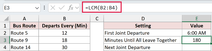
The result is 180 minutes. That’s the shortest shared interval for routes departing every 12, 18, and 30 minutes.
Even though the argument is a range, LCM returns one answer. It doesn’t spill a separate answer for each route.
To turn that interval into a departure time, enter this in E4:
=E2+E3/1440
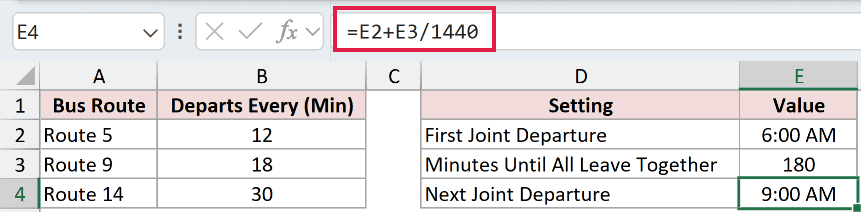
The formula converts the interval from minutes into Excel’s day-based time units, then adds it to the 6:00 AM starting time. E4 displays 9:00 AM.
Pro Tip: This scheduling method assumes the routes share a starting departure. LCM finds their repeat interval; it doesn’t account for different starting times.
Example 2: Match Different Pack Sizes
Pack sizes often leave you with more of one item than its matching partner.
Below is the dataset. Columns A:D list paired supplies and pack sizes. Columns E:G have result headers, while I:J shows the mistake of combining all pack sizes.

We want the smallest matching quantity for each pair, followed by the packs needed to buy it.
Enter this formula in E2, then copy it down through E6:
=LCM(B2,D2)

Hot dogs and buns need 40 units each. The remaining pairs return 60, 48, 24, and 200 units, respectively.
Each row gets its own LCM calculation. Filling down keeps unrelated pairs separate.
To calculate packs of item A, enter this in F2:
=E2:E6/B2:B6

This division formula spills into F2:F6, returning 4, 5, 3, 4, and 8 packs.
These division spills work in Excel 2021, Excel 2024, and Microsoft 365. In Excel 2019 and earlier, calculate each row’s division separately and fill down.
For packs of item B, enter this in G2:
=E2:E6/D2:D6

The formula spills into G2:G6, returning 5, 3, 2, 3, and 5 packs. For hot dogs and buns, that’s 4 hot-dog packs and 5 bun packs.
The mistake demonstrated in J2 is passing both complete pack-size ranges to LCM:
=LCM(B2:B6,D2:D6)

This mistake returns 1,200, the common quantity across all ten pack sizes. Each pair needs its own calculation.
Example 3: Add Fractions With a Common Denominator
LCM can put fractional recipe measurements over the same denominator before you add them.
Below is the dataset. Ingredients have separate numerator and denominator columns. Column D is reserved for scaled numerators, and F:G contains labeled cells for the denominator and totals.

We want to add the listed cup measurements while keeping a fraction representation of the total.
Find the common denominator in G2:
=LCM(C2:C5)
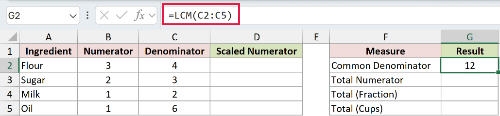
LCM returns 12, the smallest common multiple of the denominators in column C.
Scale the numerators by entering this in D2:
=B2:B5*G2/C2:C5
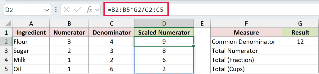
The results spill into D2:D5: 9, 8, 6, and 2. Each numerator is multiplied by the common denominator divided by its original denominator.
Add the scaled numerators in G3:
=SUM(D2:D5)
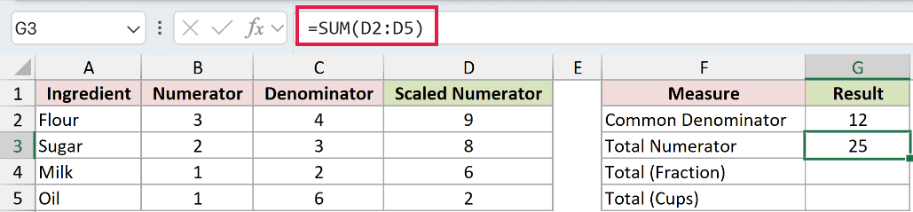
The total numerator is 25. The denominator stays 12 because all the measurements now use the same denominator.
Build the fraction label in G4:
=G3&"/"&G2
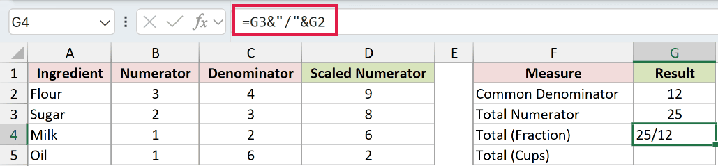
This returns 25/12 as text. It’s a readable label, so use the numeric result below for further calculations.
Calculate that numeric total in G5:
=G3/G2
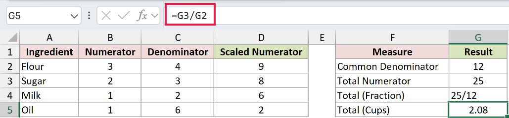
The cell displays 2.08 cups with its decimal number format.
Example 4: Schedule Checks for a Selected Line
When a list contains several production lines, filter the intervals before calculating their LCM.
Below is the dataset. Columns A:C list lines, checks, and intervals. The E:F card contains the selected line, last check date, and labeled result cells.
The last-check input in F3 uses =DATE(2026,9,1) and displays Sep 1, 2026. F2 contains the selected line, Line B.
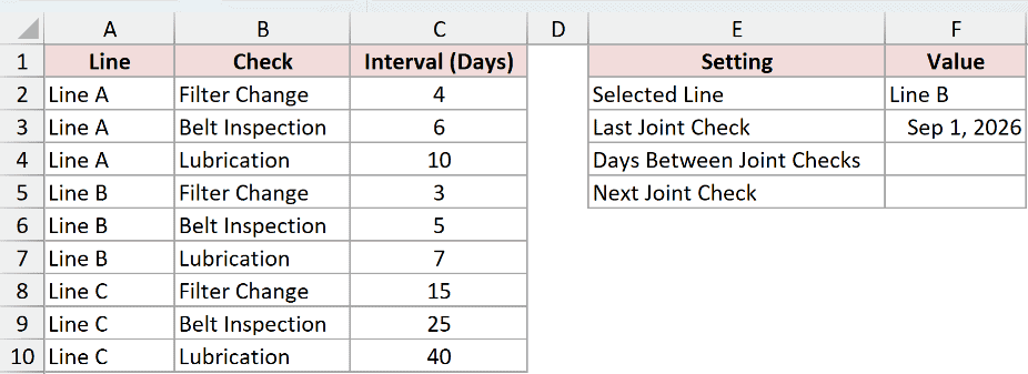
We want the next date when every check for the selected line is due together.
Enter this formula in F4:
=LCM(FILTER($C$2:$C$10,$A$2:$A$10=F2))
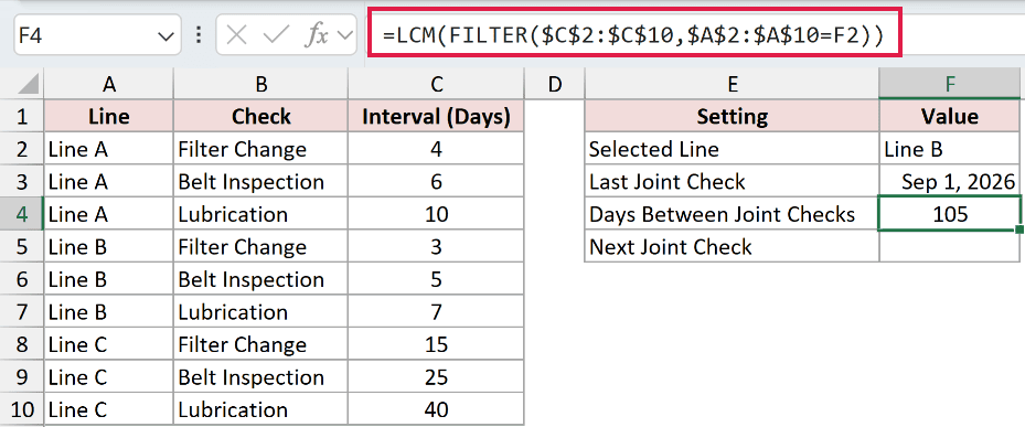
The result is 105 days for Line B.
How this formula works:
- FILTER keeps the intervals whose line label matches
F2. - For Line B, those intervals are 3, 5, and 7 days.
- LCM calculates the joint interval from those filtered numbers.
FILTER requires Excel 2021 or later. The dollar signs keep the source ranges fixed.
Calculate the next joint check in F5:
=F3+F4
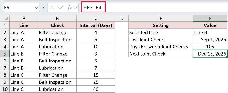
Adding the interval to the last joint check returns Dec 15, 2026. Changing the selected line changes which intervals feed LCM.
Example 5: Handle Decimal Intervals Correctly
Decimal intervals need an extra step because LCM drops their fractional parts.
Below is the dataset. Columns A:B contain pool tasks and intervals in hours. Columns D:E provide labeled cells for the plain-LCM mistake and the scaled fix.

We want the joint repeat interval without changing the original task frequencies.
The mistake in E2 is using LCM directly on the decimal hours:
=LCM(B2:B4)
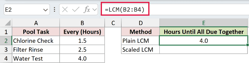
The wrong result displays as 4.0 hours. LCM truncates the inputs before calculating, so this result doesn’t represent the actual pool schedule.
The fix in E3 scales the inputs before LCM runs:
=LCM(B2:B4*10)/10
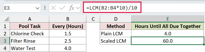
This returns 60.0 hours. Multiplication by 10 converts the intervals to whole-number tenths of an hour; division by 10 converts the LCM back to hours.
Pro Tip: Choose a scale that makes every interval a whole number before LCM evaluates it. Changing the cell’s number format alone won’t preserve fractional inputs.
Example 6: Check Blanks, Zeros, and Invalid Inputs
A blank cell and a typed zero have different effects on LCM.
Below is the dataset. Columns A:B hold input pairs, column C is reserved for each LCM result, and column D describes the behavior being tested.
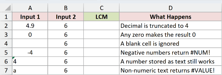
We want to see how LCM handles each input case separately.
Enter this formula in C2, then copy it down through C7:
=LCM(A2,B2)
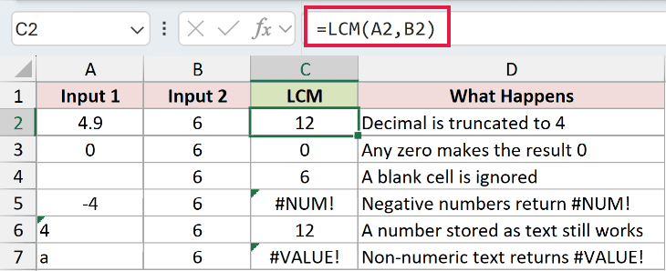
Each row tests a different case:
- Decimal:
A2contains 4.9, which LCM truncates to 4. With 6, the result inC2is 12. - Zero:
A3contains 0, soC3returns 0. - Blank:
A4is empty. LCM ignores it, leaving the other input, soC4returns 6. - Negative number:
A5contains -4, soC5deliberately returns #NUM!. Correct the negative input before using it as an interval. - Number stored as text:
A6holds text 4, which LCM accepts.C6returns 12. - Nonnumeric text:
A7holds a, soC7deliberately returns #VALUE!. Replace the text with a valid numeric input.
A numeric result can hide missing inputs because LCM ignores blank cells.
Tips & Common Mistakes
- Keep the units consistent. Convert intervals to the same unit before finding their common multiple.
- Choose the calculation scope first. LCM pools all supplied numbers. Use separate row calculations when each pair needs an independent answer.
- GCD returns the largest number that divides every input evenly. LCM finds the smallest shared multiple instead.
For positive number pairs, multiplying the inputs and dividing by their GCD also finds their LCM.
- Large calculations can overflow. LCM can return
#NUM!even with positive inputs when the calculation becomes too large. - Check missing intervals before trusting a schedule. Blanks are ignored, while a typed zero makes the result zero.
Related Excel Functions / Articles:
