How to Create a Multiplication Formula in Excel (4 Easy Ways)

If you want to multiply numbers in Excel, there’s no dedicated “times” button like a calculator has. Instead, you build a small formula and let Excel do the math for you.

The good news is that multiplying is one of the easiest things to do in Excel, and you have a few ways to go about it depending on your data.

In this guide I’ll walk through the asterisk operator, the PRODUCT function, a no-formula Paste Special trick, and a Power Query approach.

Table of Contents

Method #1: Using the Asterisk (*) Operator

The most direct way to multiply in Excel is the asterisk (*) operator. It works exactly like a times sign, so =5*3 gives you 15.

This is the method I reach for most often, since it reads cleanly and you can point it at any cells you want.

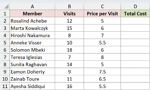
Below I have a dataset of gym member check-ins. Each row has the number of visits and the price per visit, and I want the total cost for every member.

Gym member check-ins with visits in column B and price per visit in column C, ready for a Total Cost in column D

Here is the formula I’ll put in cell D2:

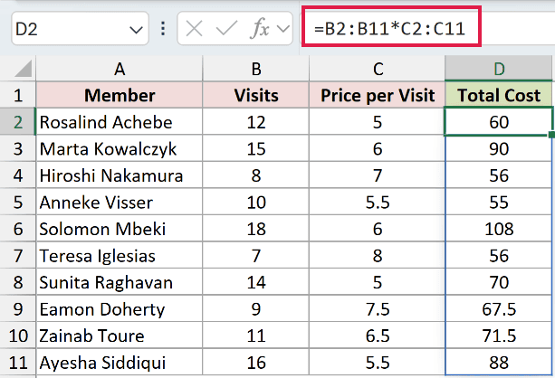
=B2:B11*C2:C11

=B2:B11*C2:C11 typed once in cell D2 and spilling a total for every member down column D

How does this formula work?

I’m multiplying the whole Visits range (B2:B11) by the whole Price per Visit range (C2:C11) in one shot. Excel pairs up each row, so B2 multiplies with C2, B3 with C3, and so on.

Because this is a dynamic array formula, the result spills down the column automatically. I only type it once in D2 and every total below fills in on its own.

For Rosalind Achebe that’s 12 visits at $5, which returns 60. Marta Kowalczyk has 15 visits at $6, so the total comes to 90.

Note: If you’re on an older version of Excel that doesn’t support spilling, use =B2*C2 in the first cell instead and drag it down the column.

Method #2: Using the PRODUCT Function

If you’d rather use a function than an operator, PRODUCT does the same job. It multiplies all the numbers you give it, whether that’s two cells or a whole range of them.

PRODUCT really shines when you have several values to multiply together, since you can hand it a range instead of chaining a long string of asterisks.

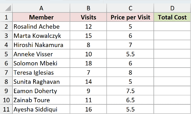
I’m using the same gym check-in data here. Each member has a visit count and a price per visit, and I want the total cost.

The same gym check-in data with an empty Total Cost column, this time for the PRODUCT function

Here is the formula I’ll enter in cell D2:

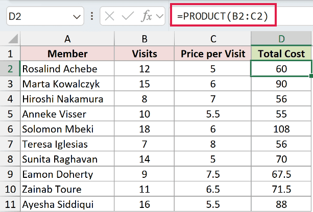
=PRODUCT(B2:C2)

=PRODUCT(B2:C2) in cell D2 returning 60 for 12 visits at $5 each

How does this formula work?

PRODUCT looks at the range B2:C2 and multiplies everything inside it. For row 2 that’s 12 times 5, which returns 60.

Since PRODUCT collapses a range into a single value, it doesn’t spill on its own. I enter it in D2 and then copy it down for the rest of the members.

The handy part is the range argument. If you later add more factors, say a discount column inserted before Total Cost (which pushes the totals over to column E), you can widen the formula to =PRODUCT(B2:D2) without rewriting it with extra asterisks.

Method #3: Using Paste Special (No Formula Needed)

Sometimes you don’t want a formula at all. You just want to scale a set of numbers in place, and Paste Special can do that.

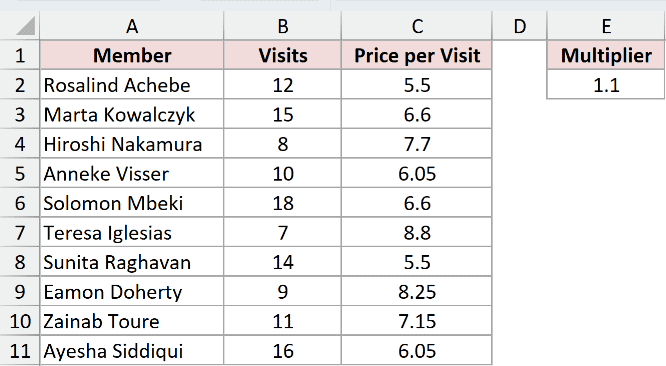
Say the gym raises the price of every visit by 10%. Instead of building a formula and then converting it back to values, I can multiply the existing prices by 1.1 directly.

Here is the Price per Visit column I want to bump up by 10%.

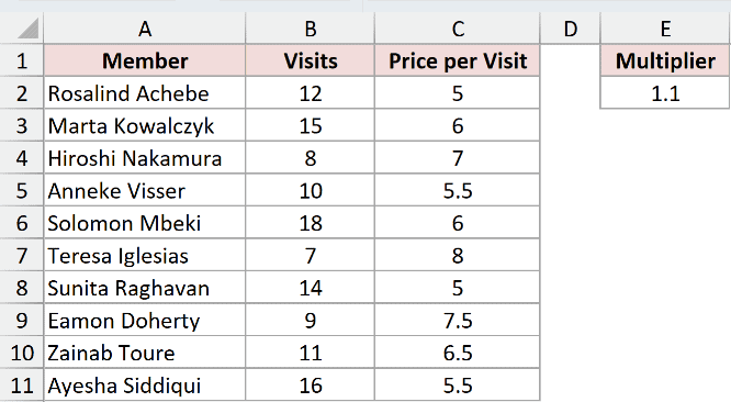
The price per visit column alongside a multiplier of 1.1 parked in cell E2

Here are the steps to multiply the values using Paste Special:

In any empty cell, type the number you want to multiply by (here I typed 1.1), then copy it with Control + C.

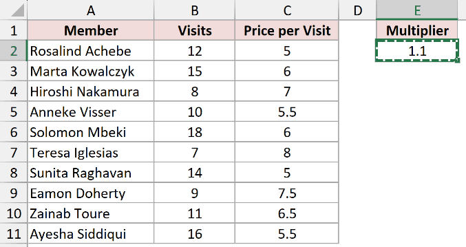
The multiplier 1.1 in cell E2 copied, with the marching ants border showing it is on the clipboard

Select the range of prices you want to change (C2:C11).

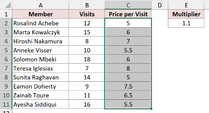
The ten price cells C2 to C11 selected, ready to be multiplied in place

Right-click the selection and choose Paste Special. You can also press Ctrl + Alt + V on Windows or Command + Control + V on Mac.

In the dialog box, select Multiply under Operation, then click OK.

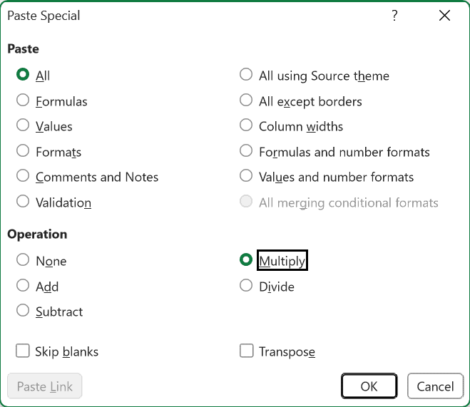
The Paste Special dialog with Multiply selected under Operation

Every price is now multiplied by 1.1 right where it sits. A $5 visit becomes $5.50 and an $8 visit becomes $8.80, with no formula left behind.

Every price multiplied by 1.1 in place, with $5 now reading 5.5 and $8 reading 8.8, and the 1.1 multiplier still sitting in E2

Note: Paste Special overwrites the original numbers in place, so this can’t be undone once you save and close. Keep a copy of the source data if you might need the pre-multiplied values.

Method #4: Using Power Query

If your multiplication is part of a larger data cleanup, Power Query lets you add a calculated column as a repeatable step. Refresh the query later and the new data flows through the same math.

This one is more setup than a plain formula, so I reach for it when I’m already shaping data in Power Query, not for a one-off multiply.

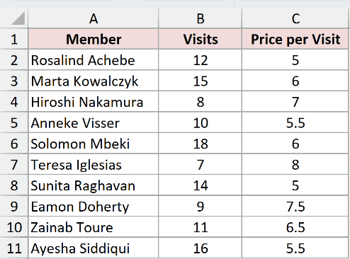
Here is the gym check-in data I’ll load. I want a Total Cost column that multiplies Visits by Price per Visit.

The gym check-in data that will be loaded into Power Query, with visits and price per visit

Here are the steps to multiply two columns in Power Query:

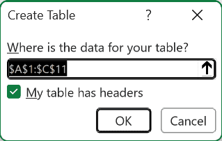
Select any cell in the data and press Control + T to convert it into an Excel Table, then click OK.

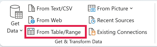
The Create Table dialog after pressing Control + T, with the whole data range detected and headers ticked

With the table selected, go to the Data tab and click From Table/Range to open the Power Query Editor.

The From Table/Range button on the Data tab, which opens the Power Query Editor

In the editor, go to the Add Column tab and click Custom Column.

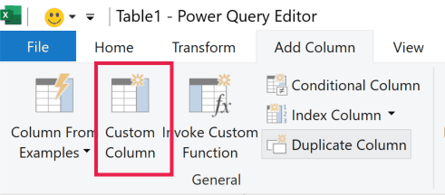
Power Query Editor Add Column tab with the Custom Column button highlighted by a red box

Name the column Total Cost and enter the formula below, then click OK.

[Visits] * [Price per Visit]

Custom Column dialog box showing the formula [Visits] * [Price per Visit] to calculate Total Cost

Go to the Home tab and click Close & Load to send the result to a new sheet.

Power Query loads a new table with the Total Cost column filled in. The math lives as a saved step, so it runs again whenever you refresh.

Note: Power Query doesn’t update on its own. When the source data changes, go to the Data tab and click Refresh All to rerun the multiplication.

Additional Notes About Multiplying in Excel

Lock a fixed multiplier with dollar signs. When you multiply a column by one fixed cell, use an absolute reference like =B2*$F$1 so the multiplier doesn’t shift as you copy the formula down.
Watch for text that looks like a number. A “number” stored as text (often left-aligned or with a stray space) will trip up your formula. Convert it to a real number first, or the result won’t add up.
Mind the order of operations. Excel does multiplication before addition, so =B2+C2*D2 may not be what you meant. Wrap the part you want done first in parentheses.
Multiplying by a percentage is just multiplying by a decimal. To take 20% of a value, multiply by 0.2. Formatting a cell as a percent doesn’t change the math underneath.

Frequently Asked Questions

Why is my multiplication formula returning a #VALUE! error?

Excel returns #VALUE! when one of the cells you’re multiplying holds text instead of a number. Check for stray letters, spaces, or numbers stored as text, then fix the value or use a helper column to convert it.

Can I multiply an entire column by the same fixed number?

Yes. Put the fixed number in a cell, then write a formula like =B2*$F$1 with dollar signs on the fixed cell and copy it down. The $F$1 reference stays locked while B2 moves with each row.

How do I multiply cells that are on two different sheets?

Reference the sheet name in the formula. For example, =Sheet1!B2*Sheet2!B2 multiplies cell B2 on Sheet1 by cell B2 on Sheet2. Excel adds the sheet reference automatically if you click the cells while building the formula.

Conclusion

Multiplying in Excel comes down to picking the right tool for the job. For everyday math, the asterisk operator is the fastest and clearest choice, and PRODUCT is handy when you’re multiplying a whole range at once.

Reach for Paste Special when you want to scale existing numbers in place, and Power Query when the multiplication is one step in a bigger, repeatable workflow.

Other Excel articles you may also like: