
The RECEIVED function in Excel returns the amount paid at maturity for a fully invested security bought at a discount rate.
You enter the money paid upfront, the quoted discount rate, and the purchase and maturity dates. The result includes your original investment and the gain.
This suits commercial paper, where a company borrows money through a short-term security and repays it at maturity. The quoted discount rate determines the gap between purchase and repayment.
I’ll show you how to calculate repayments and see how different discount rates affect the amount you receive.
RECEIVED Function Syntax in Excel
RECEIVED takes the purchase details and an optional day count basis:
=RECEIVED(settlement, maturity, investment, discount, [basis])
- settlement (required): The date you purchase the security. Use a real Excel date.
- maturity (required): The date the security pays out. It must come after settlement.
- investment (required): The amount you pay upfront, entered as a positive amount.
- discount (required): The annual discount rate. Enter a percentage, such as
4.60%, rather than a whole-number rate. - basis (optional): The day count method. Omitting it uses
0, US (NASD) 30/360. Example 3 compares all the available methods.
The discount applies to the maturity amount. RECEIVED works backward from the amount invested to find that maturity amount.
When to Use RECEIVED Function
- Calculate the cash repayment for commercial paper bought at a quoted discount rate.
- Work out maturity amounts for purchases with different terms and investment sizes.
- Check how the contract’s day count method affects the payout.
- Compare discount-rate scenarios while keeping the purchase amount and dates fixed.
Example 1: Calculate the Amount at Maturity
Let’s start with a single commercial-paper purchase.
Below is the dataset. Cells B1:B5 hold the settlement date, maturity date, investment, discount rate, and basis. The labelled cells beneath them will hold the answers.
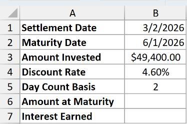
We want to find the full repayment, then separate the interest earned from the original investment.
Enter this formula in B6:
=RECEIVED(B1,B2,B3,B4,B5)
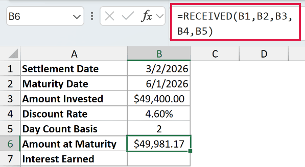
The formula returns $49,981.17 for the $49,400.00 investment at 4.60%, using the dates in B1:B2 and basis 2.
That result is the entire amount received. To find only the interest earned, enter this subtraction in B7:
=B6-B3
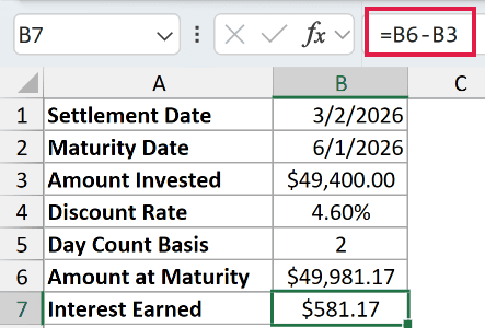
B7 returns $581.17. Subtracting the original investment keeps the maturity payout separate from the gain.
Basis 2 means Actual/360. RECEIVED counts the actual days between the dates and divides that count by a 360-day year.
Example 2: Calculate Repayments for Different Terms
A purchase list often specifies a term in days instead of a maturity date.
Below is the dataset. Columns A:D list fictional issuers, terms, investments, and discount rates. The side card holds the shared purchase date and basis.

We want each purchase’s maturity amount in column E, calculating its maturity date from its term.
Enter this formula in E2, then copy it down through E6:
=RECEIVED($H$2,$H$2+B2,C2,D2,$H$3)
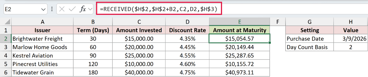
The formula adds the term in B2 to the purchase date in H2. That calculated date becomes RECEIVED’s maturity argument.
The dollar signs lock H2 and H3 while the term, investment, and discount references move with each row.
Brightwater Freight’s 30-day purchase returns $15,054.57 from $15,000.00 invested at 4.35%.
Tidewater Grain’s 180-day purchase returns $40,973.11 from $40,000.00 invested at 4.75%.
The repayment amounts reflect different investment sizes as well as rates and terms.
Example 3: Compare Day Count Methods
The basis argument can change the answer even when every other input stays the same.
Below is the dataset. Columns A:B list basis codes and methods. The side card in E:F contains the note’s dates, investment, and discount rate.
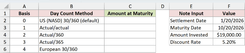
We want to isolate the effect of each day count method on the maturity amount.
Enter this formula in C2 and copy it down through C6:
=RECEIVED($F$2,$F$3,$F$4,$F$5,A2)
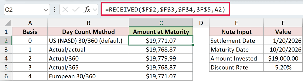
The locked references keep the note details fixed. Only the basis reference changes as you copy down.
For the $19,000.00 investment at 5.20%, the workbook returns:
- 0, US (NASD) 30/360: $19,771.07.
- 1, Actual/actual: $19,768.87.
- 2, Actual/360: $19,779.99.
- 3, Actual/365: $19,768.87.
- 4, European 30/360: $19,771.07.
Some methods agree for these dates. Use the method specified for your purchase.
Pro Tip: Use the basis stated in the security’s terms. Leaving basis out selects US (NASD) 30/360; it doesn’t ask Excel to detect the appropriate method.
Example 4: Separate Discount Rate From Investment Return
The quoted discount rate isn’t the annual return on the cash you actually invest.
Below is the dataset. B1:B5 contains the dates, investment, quoted discount rate, and basis. The labelled answer cells will show the maturity amount and annual return.
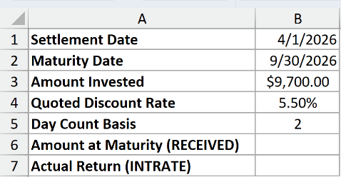
We want the maturity amount first, then the annual return implied by that repayment.
Enter the RECEIVED formula in B6:
=RECEIVED(B1,B2,B3,B4,B5)
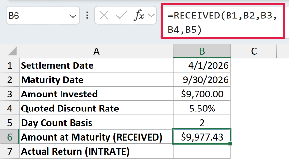
RECEIVED returns $9,977.43 for the $9,700.00 investment and the quoted 5.50% discount rate.
INTRATE calculates a simple annual interest rate from the investment and repayment. Here, it uses RECEIVED’s result to express the gain relative to the cash invested.
Enter this formula in B7:
=INTRATE(B1,B2,B3,B6,B5)
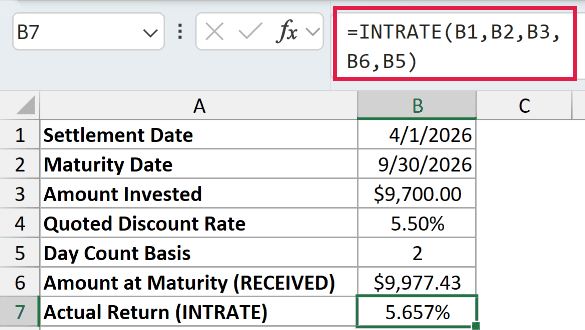
The annual return is 5.657%, above the 5.50% discount rate.
The discount rate measures the gain against the maturity amount. The investment return measures that gain against the smaller amount paid upfront, so the percentage is higher.
B7 is an annualized rate using the specified basis. It isn’t the percentage earned over the holding period or a compounded annual return.
Example 5: Compare Discount Rates With One Formula
Now let’s hold the purchase details steady and change only the quoted rate.
Below is the dataset. A2:A7 contains discount rates, and the card in D:E holds the settlement date, maturity date, investment, and basis.
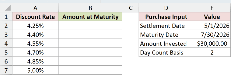
We want a maturity amount beside every rate without copying the formula down.
Enter this formula in B2:
=RECEIVED(E2,E3,E4,+A2:A7,E5)
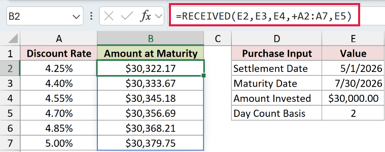
The leading + converts the range into an array of numeric values RECEIVED can process. Passing the bare range instead returns a single #VALUE! error.
The results spill from B2 through B7. Enter the formula only in B2; Excel fills the remaining result cells automatically.
This spill works in Excel 2021, Excel 2024, and Microsoft 365. In Excel 2019 and earlier, use individual rate references and copy down, as in Example 2.
With $30,000.00 invested, the 4.25% scenario returns $30,322.17. The 5.00% scenario returns $30,379.75.
With the investment and dates held fixed, increasing the discount rate raises the maturity amount.
Example 6: Diagnose RECEIVED Errors
Let’s finish with a working purchase and deliberate input mistakes.
Below is the dataset. Column A describes each case, and B:F contains its dates, investment, rate, and basis. Column G will show the result or error.
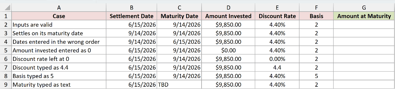
We want to see which input causes each error so we can correct the source value.
Enter this formula in G2 and copy it down through G9:
=RECEIVED(B2,C2,D2,E2,F2)
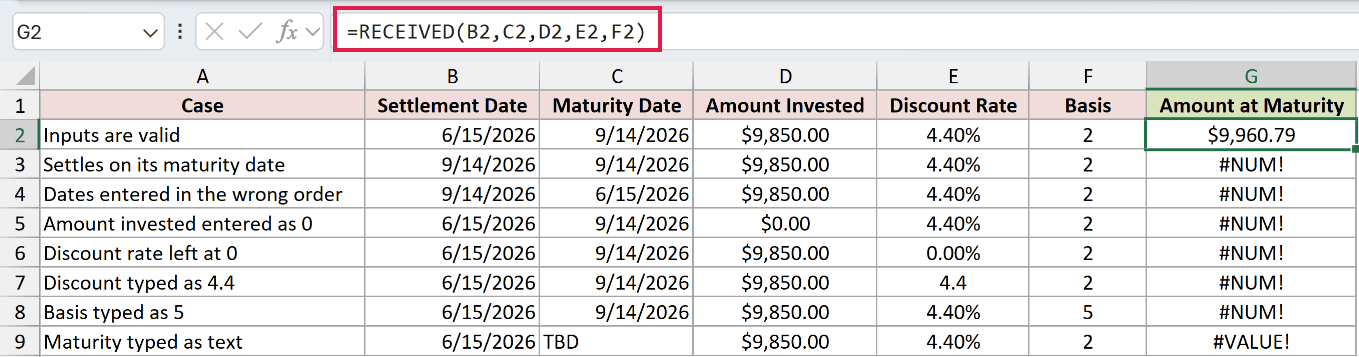
The valid case in G2 returns $9,960.79. The rows underneath deliberately demonstrate input errors.
- G3 returns
#NUM!: Settlement equals maturity. Settlement must come earlier. - G4 returns
#NUM!: The dates are reversed. Correct the settlement and maturity entries. - G5 returns
#NUM!: The investment is $0.00. Enter the positive amount paid for the security. - G6 returns
#NUM!: The discount rate is 0.00%. RECEIVED requires a positive discount rate. - G7 returns
#NUM!: The rate was typed as 4.4. Enter 4.40%, including the percent sign, for the intended quote. - G8 returns
#NUM!: Basis 5 isn’t supported. Choose the applicable code from Example 3. - G9 returns
#VALUE!: The maturity cell contains TBD, not a date. Replace it with the actual maturity date.
Tips & Common Mistakes
- Keep the quote type straight. RECEIVED expects a discount rate. Don’t substitute an annual investment-return percentage into that argument.
- Use whole-number basis codes. In testing, basis 1.9 behaved like basis 1 because Excel truncated it.
- Don’t use RECEIVED as a compound-growth model. It uses simple discounting. In testing, a 12-year term at 10% returned
#NUM!because the rate multiplied by the time exceeded 1. - Format the payout as currency. RECEIVED returns a money amount; the percentage formatting belongs on the rate inputs and the annual-return comparison.
- Check the underlying inputs before hiding an error. A missing date or incorrectly entered rate needs correction before the maturity amount can be used.
Related Excel Functions / Articles:
