
The YIELDMAT function in Excel returns the annual yield of a security that pays interest at maturity.
Its rate argument is the interest rate set at issue. The returned yield also reflects the buyer’s settlement date, purchase price, and chosen day-count basis.
In this article, I’ll show you how to normalize price, spill several yields, compare basis and price effects, and recognize invalid inputs.
YIELDMAT Function Syntax in Excel
The YIELDMAT function uses five required arguments and one optional day-count basis.
=YIELDMAT(settlement, maturity, issue, rate, pr, [basis])
- settlement (required) is the date the buyer acquires the security after its issue date. It is the settlement date, which is not necessarily the trade date.
- maturity (required) is the date the security expires and pays its maturity amount.
- issue (required) is the date the security was issued.
- rate (required) is the security’s interest rate at the issue date. It is an input, not the annual yield returned by YIELDMAT.
- pr (required) is the security’s price per $100 of face value.
- basis (optional) sets the day-count convention. Use
0or omit it for US (NASD) 30/360,1for Actual/actual,2for Actual/360,3for Actual/365, or4for European 30/360.
When to Use YIELDMAT Function
- Calculate annual yield for a security that pays interest at maturity.
- Convert a whole-position purchase cost into the price per $100 required by the function.
- Compare yields across several maturity-interest securities.
- Test how day-count basis or purchase price changes the annual yield.
- Check whether invalid dates, rates, prices, or basis codes are causing errors.
Example 1: Normalize Price Before Using YIELDMAT
Start with a single maturity-interest security purchased below face value.
Below is the dataset. It contains the dates, issue rate, face value, total clean purchase price, and basis. The price and yield result cells are empty.
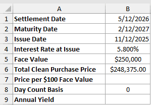
We first want to convert the total purchase price into a price per $100 in B7.
Enter this formula in B7:
=B6/B5*100
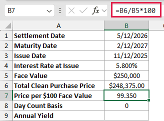
The $248,375 clean price is 99.35% of the $250,000 face value, so B7 returns 99.350.
We now want the annual yield in B9.
Enter this formula in B9:
=YIELDMAT(B1,B2,B3,B4,B7,B8)
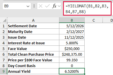
YIELDMAT uses the normalized price with the three dates, issue rate, and basis. The annual yield is 6.5200%.
That differs from the 5.800% issue rate because yield also reflects the below-par purchase price and the time remaining until maturity.
Pro Tip: The pr argument is price per $100 of face value. Do not pass the total cost of the whole position.
Example 2: Spill Yields for Several Securities
One array formula can calculate a small security report.
Below is the dataset. Each row has its own dates, rate, price per $100, and basis. The Annual Yield column is empty.

We want one annual yield for every security in H2:H7.
Enter this formula in H2 and let it spill through H7:
=YIELDMAT(+B2:B7,+C2:C7,+D2:D7,+E2:E7,+F2:F7,+G2:G7)
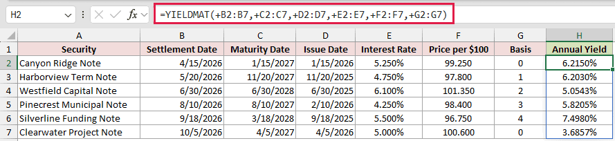
The unary plus signs convert each direct range reference into a value array. YIELDMAT then evaluates corresponding rows and spills six yields.
Direct multi-cell references without unary plus return #VALUE!. The coercion is required here; it is not decorative formula syntax.
Canyon Ridge returns 6.2150%. Silverline is highest at 7.4980%, while Clearwater is lowest at 3.6857%.
Pro Tip: This spilling form works in Excel 2021, Excel 2024, and Microsoft 365. In Excel 2019 or earlier, use one scalar YIELDMAT formula per row.
Example 3: Compare All Day-Count Bases
Day-count basis can change the annualized result.
Below is the dataset. A shared security card sits beside basis codes 0 through 4 and their convention names. The Annual Yield column is empty.
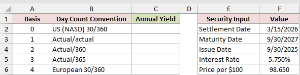
We want to calculate the yield under every supported basis in C2:C6.
Enter this formula in C2 and let it spill through C6:
=YIELDMAT($F$2,$F$3,$F$4,$F$5,$F$6,+A2:A6)
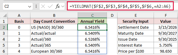
The fixed F references keep the security inputs constant. Unary plus turns A2:A6 into the value array that supplies each basis code.
Basis 0 and 4 return 6.5416%. Basis 1 and 3 return 6.5409%, while basis 2 returns 6.5268%.
Choose the basis specified for the security. A numerically valid code can still produce the wrong answer if it represents the wrong convention.
Example 4: See How Price Changes Yield
Now keep every input except purchase price constant.
Below is the dataset. Three rows use the same dates, issue rate, and basis with discount, near-par, and premium prices. Annual Yield is empty.

We want the annual yield for each price scenario in H2:H4.
Enter this formula in H2 and let it spill through H4:
=YIELDMAT(+B2:B4,+C2:C4,+D2:D4,+E2:E4,+F2:F4,+G2:G4)

The price of 96.000 returns 6.7323%. Raising the price to 99.500 lowers the yield to 5.3968%.
At the premium price of 102.500, the yield falls to 4.3210%. A buyer paying more for the same maturity payment earns a lower annual yield.
Example 5: Recognize Intentional YIELDMAT Errors
These rows deliberately test YIELDMAT’s documented error conditions.
Below is the dataset. The first row is valid. The remaining rows each contain one invalid input, and the YIELDMAT Result column is empty.

We want to calculate every row and see which input conditions fail in H2:H7.
Enter this formula in H2, then copy it down through H7:
=YIELDMAT(B2,C2,D2,E2,F2,G2)
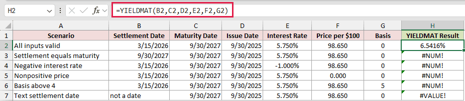
The first row returns the valid yield 6.5416%. The next five outcomes are intentional checks, not broken formulas.
- Settlement equal to maturity returns
#NUM!. - A negative issue rate returns
#NUM!. - A price of zero returns
#NUM!. - Basis 5 returns
#NUM!because only 0 through 4 are supported. - A text settlement date returns
#VALUE!.
Pro Tip: Store settlement, maturity, and issue as real Excel dates. A date that only looks valid because it is text can still return #VALUE!.
Tips & Common Mistakes
- Use YIELDMAT only when the security pays interest at maturity. Use YIELD for a security that pays periodic interest.
- Treat settlement as the buyer’s acquisition or settlement date after issue. Do not assume it is always the trade date.
- Keep the issue rate and annual yield separate. The rate is an input, while YIELDMAT calculates yield from the full set of terms.
- Pass price per $100 face value to
pr, not a whole-position purchase cost. - Basis accepts only 0 through 4. If omitted, Excel uses US (NASD) 30/360.
- Excel truncates settlement, maturity, issue, and basis to integers. Time components in the date serial numbers do not affect YIELDMAT.
- Direct multi-cell range references return
#VALUE!in YIELDMAT. Add unary plus to each range when you need a spilling value-array calculation. - Settlement must be earlier than maturity. Rates cannot be negative, and price must be greater than zero.
I have shown how to calculate YIELDMAT from normalized prices, spill multiple yields, compare basis and price effects, and diagnose invalid inputs.
I hope you found this article helpful.
Related Excel Functions / Articles:
