How to Do a Fuzzy Lookup in Excel

Misspelled names and inconsistent spacing can turn an ordinary lookup into a blank result, even when both records refer to the same place or person.

A fuzzy lookup compares text by similarity, so you can connect entries that aren’t identical.

Excel has no FUZZYMATCH function. Power Query is the best choice for most lists, while wildcards and VBA cover narrower cases.

Method #1: Using Power Query Fuzzy Merge

Power Query’s fuzzy merge is the method I recommend for most readers. It compares text with the Jaccard similarity algorithm and can return the closest qualifying match.

Below I have entry IDs and typed city names in A1:B11, plus the official city list in D1:D9. I want to match each entry to an official city.

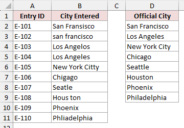
Power Query fuzzy matching works only with text columns. Both source ranges must also be Excel Tables before you load them into Power Query.

Here are the steps to create the fuzzy merge:

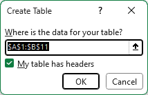
1. Select each source range and press Ctrl + T to turn it into an Excel Table.

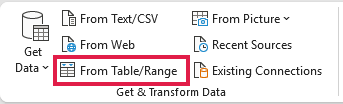
2. Select a cell in each table and use Data > From Table/Range to create a query for each one.

3. In the Power Query Editor, select the city-entry query. On the Home tab, choose Merge Queries > Merge Queries as New.

4. Select the two queries and their city columns. Check Use fuzzy matching to perform the merge.

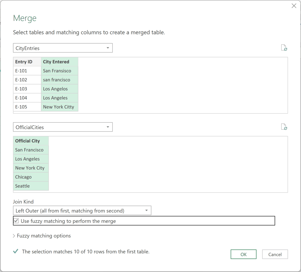
5. Open Fuzzy matching options and review these settings:

• Similarity threshold (optional): Start at the default 0.80. The allowed range is 0.00 to 1.00.
• Ignore case: Keep this on when capitalization shouldn’t affect a match.
• Match by combining text parts: This is IgnoreSpace in M. It can match “Micro soft” to “Microsoft”, but not “M 365” to “M365”.
• Maximum number of matches (optional): Set this to 1 when you want one closest match for each entry.
• Transformation table (optional): Choose a query with From and To columns when you need controlled substitutions.

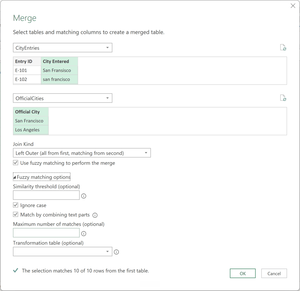
The threshold is a lower limit. A threshold of 1.00 allows exact matches only, while 0.00 allows everything to qualify.

I start at the default 0.80 and check the loaded result for blank rows. I lower the threshold only when a real match was missed.

6. Click OK to run the fuzzy merge.

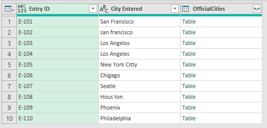
Entries that score below the chosen threshold return a blank match. Power Query returns the closest match that clears the threshold.

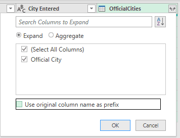
7. Expand the merged column, tick Official City, and untick Use original column name as prefix.

8. On the Home tab, click Close & Load to place the result in a new table on a worksheet.

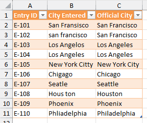
At the default 0.80 threshold, all ten entries matched. The dialog footer confirmed, “The selection matches 10 of 10 rows from the first table.”

San Fransisco, Los Angelos, New York Citty, Chigago, Seatle, and Phliadelphia all resolved to the correct official cities.

“Hous ton” matched Houston because Match by combining text parts is on by default. “san francisco” matched because Ignore case is on by default.

Every messy entry cleared the default threshold comfortably, so 0.80 is a sensible starting point rather than a number to change straight away.

Note: A transformation-table match carries a deliberate 0.05 penalty, so its score cannot exceed 0.95. To avoid that penalty, replace the column values first and then run the fuzzy match.

Method #2: Using Wildcards With XLOOKUP

Here’s a formula option when the shorter text already appears intact inside the full name. It is useful for partial names, but it isn’t true fuzzy matching.

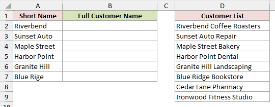
Below I have short customer names in A2:A7 and a full customer list in D2:D9. I want to return the full name in column B.

Note: XLOOKUP requires Excel 2021, Microsoft 365, or Excel 2024. Excel 2016 and 2019 do not have it, so use VLOOKUP with the same asterisk wildcards instead.

Enter this formula in B2 and fill it down to B7:

=XLOOKUP("*"&A2&"*",$D$2:$D$9,$D$2:$D$9,"Not found",2)

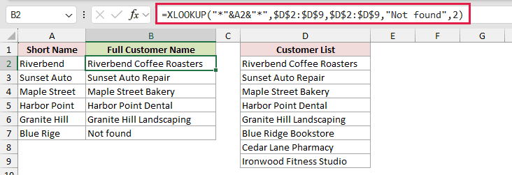
The asterisks around A2 let extra text appear before or after the short name. XLOOKUP’s fifth argument is 2, which switches on wildcard matching.

The formula searches D2:D9 and returns the matching full customer name from that same range. If no substring matches, it returns “Not found”.

The first five short names return their corresponding full customer names. “Blue Rige” returns “Not found” because it is a typo, not an intact substring.

Wildcards match substrings, not misspellings. Use Power Query when the text itself contains spelling differences.

Method #3: Using Table.FuzzyGroup in the Advanced Editor

Here’s another way to handle duplicates in one column: Table.FuzzyGroup can collect similar supplier names and count the invoices in each group.

The Group By dialog’s fuzzy grouping checkbox is available only in Power Query Online. In Excel desktop, you use the same feature through the Advanced Editor.

Below I have invoice IDs and supplier names in A1:B11 on the Fuzzy Group sheet. I want to collapse spelling and capitalization variants without changing the source invoices.

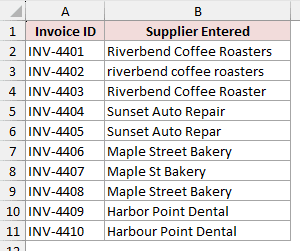
The code expects the Excel Table to be named Suppliers and uses Source because From Table/Range creates the first query step with that name.

Here are the steps to group the supplier names:

1. Select A1:B11 on the Fuzzy Group sheet, press Ctrl + T to create an Excel Table, and name the table Suppliers.

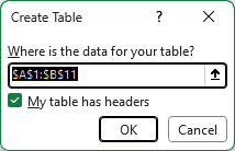
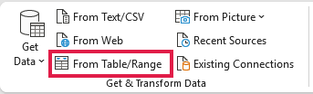
2. Select a cell in the table, then choose Data > From Table/Range to load it into the Power Query Editor.

3. On the Home tab, click Advanced Editor.

4. Replace the existing query code with the code below. It uses Source, sets Supplier Entered to text in Typed, and returns Grouped as the final step.

Fuzzy matching works only on columns Excel knows are text. Reading a table straight from the workbook leaves its columns untyped, so the Typed step is required.

let
    Source = Excel.CurrentWorkbook(){[Name="Suppliers"]}[Content],
    Typed = Table.TransformColumnTypes(Source, {{"Supplier Entered", type text}}),
    Grouped = Table.FuzzyGroup(
        Typed,
        "Supplier Entered",
        {{"Invoice Count", each Table.RowCount(_)}},
        [IgnoreCase = true,
         IgnoreSpace = true,
         Threshold = 0.8]
    )
in
    Grouped

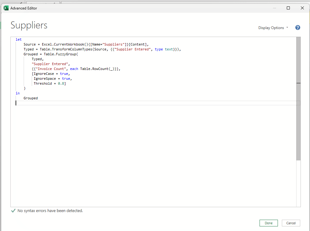
The settings inside the final record control how Power Query compares and groups the supplier names:

• Threshold: Accepts 0.00 to 1.00 and defaults to 0.80. Lower it to group more loosely.
• IgnoreCase: Defaults to true. This groups “riverbend coffee roasters” with “Riverbend Coffee Roasters”.
• IgnoreSpace: Defaults to true and combines text parts, so “Gra pes” groups with “Grapes”. It still won’t group “M 365” with “M365”.
• SimilarityColumnName: This optional setting isn’t used in the code above. It defaults to null, so no similarity column appears unless you name one.
• TransformationTable: Uses a table with From and To columns for mappings the algorithm cannot infer, such as an abbreviation.
• Culture: Defaults to "", which means Invariant English.

For each group, Power Query uses the most frequent value as the canonical one. If several values tie, it uses the first value.

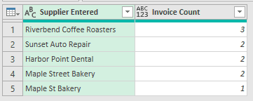
5. Close the Advanced Editor and check the grouped preview.

6. On the Home tab, click Close & Load to send the grouped result to a new table on a worksheet.

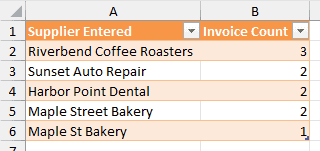
At 0.80, ten invoices collapsed into five groups.

The counts were Riverbend Coffee Roasters (3), Sunset Auto Repair (2), Harbor Point Dental (2), Maple Street Bakery (2), and Maple St Bakery (1).

“riverbend coffee roasters” and “Riverbend Coffee Roaster” both folded into “Riverbend Coffee Roasters”. “Harbour Point Dental” folded into “Harbor Point Dental”.

“Maple St Bakery” did not join “Maple Street Bakery”. The abbreviation was too far from the full word to clear 0.8.

This is where I would lower the threshold or use a transformation table to map “Maple St Bakery” to “Maple Street Bakery”.

The grouped result doesn’t replace the source rows. Power Query loads it as a separate table, so your invoice data remains intact.

Method #4: Using a VBA Similarity Function

If you need a numeric similarity percentage in worksheet cells, a VBA user-defined function gives you that control.

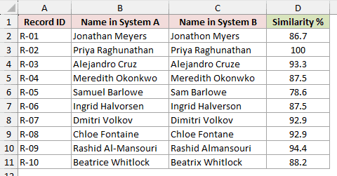
Below I have record IDs and names from two systems in columns A:C. Column D shows the verified scores produced by the function for these pairs.

Here is the VBA code:

Function SimilarityPct(text1 As String, text2 As String) As Double
    Dim a As String, b As String
    Dim i As Long, j As Long, cost As Long
    Dim d() As Long

    a = LCase(text1)
    b = LCase(text2)

    ReDim d(Len(a), Len(b))

    For i = 0 To Len(a)
        d(i, 0) = i
    Next i
    For j = 0 To Len(b)
        d(0, j) = j
    Next j

    For i = 1 To Len(a)
        For j = 1 To Len(b)
            If Mid(a, i, 1) = Mid(b, j, 1) Then
                cost = 0
            Else
                cost = 1
            End If
            d(i, j) = Application.Min(d(i - 1, j) + 1, _
                                      d(i, j - 1) + 1, _
                                      d(i - 1, j - 1) + cost)
        Next j
    Next i

    If Application.Max(Len(a), Len(b)) = 0 Then
        SimilarityPct = 100
    Else
        SimilarityPct = Round((1 - d(Len(a), Len(b)) / _
                        Application.Max(Len(a), Len(b))) * 100, 1)
    End If
End Function

Function SimilarityPct(text1 As String, text2 As String) As Double
    Dim a As String, b As String
    Dim i As Long, j As Long, cost As Long
    Dim d() As Long

    a = LCase(text1)
    b = LCase(text2)

    ReDim d(Len(a), Len(b))

    For i = 0 To Len(a)
        d(i, 0) = i
    Next i
    For j = 0 To Len(b)
        d(0, j) = j
    Next j

    For i = 1 To Len(a)
        For j = 1 To Len(b)
            If Mid(a, i, 1) = Mid(b, j, 1) Then
                cost = 0
            Else
                cost = 1
            End If
            d(i, j) = Application.Min(d(i - 1, j) + 1, _
                                      d(i, j - 1) + 1, _
                                      d(i - 1, j - 1) + cost)
        Next j
    Next i

    If Application.Max(Len(a), Len(b)) = 0 Then
        SimilarityPct = 100
    Else
        SimilarityPct = Round((1 - d(Len(a), Len(b)) / _
                        Application.Max(Len(a), Len(b))) * 100, 1)
    End If
End Function

Here are the steps to use the function:

1. Press Alt + F11 to open the VBA Editor.
2. Choose Insert > Module.
3. Paste the code into the new module.
4. Return to the worksheet and enter this formula in D2:

=SimilarityPct(B2,C2)

5. Fill the formula down the column.
6. Save the workbook as an .xlsm file to keep the macro.

The function changes both names to lowercase, calculates their Levenshtein distance, and converts that distance into a percentage rounded to one decimal place.

An exact pair such as “Priya Raghunathan” scores 100. “Samuel Barlowe” and “Sam Barlowe” score 78.6 because more of the text differs.

The approved .xlsx example stores the scores as values because that file type cannot carry the user-defined function. Add the code and save as .xlsm for live calculations.

Additional Notes About Fuzzy Lookups in Excel

• Power Query fuzzy matching supports text columns only. It doesn’t fuzzy-match number or date columns.
• Excel’s Merge dialog doesn’t show match scores. To see them, add SimilarityColumnName to the join’s options record in Advanced Editor, then expand that field with the matched column. My city scores ran from 0.94 for Seatle to 1 for case-only differences.
• Cluster values and the Group By dialog’s fuzzy grouping checkbox are available only in Power Query Online. Excel desktop has fuzzy merge in the Merge dialog and fuzzy grouping through Table.FuzzyGroup in the Advanced Editor.
• Microsoft’s old Fuzzy Lookup Add-In is retired, and its Download Center page is no longer available.
• A Marketplace listing with the same name is a third-party paid add-in from SMALLPDF KENYA. It isn’t the retired Microsoft Research add-in and was rated 1.4 out of 5 from 11 ratings when checked in September 2026.
• Power Query results don’t update automatically. Use Data > Refresh All after the source tables change.

Frequently Asked Questions

Is there a FUZZYMATCH function in Excel?

No. Excel has no native FUZZYMATCH or FUZZYLOOKUP function, despite what some articles claim.

Use Power Query for real fuzzy matching. Wildcard XLOOKUP works only when the lookup text appears as an intact substring.

Where did the Fuzzy Lookup add-in go?

Microsoft retired the Fuzzy Lookup Add-In. On September 20, 2026, its Download Center page reported that the download was no longer available in multiple regions.

Don’t confuse it with the similarly named paid Marketplace add-in from SMALLPDF KENYA. That listing isn’t Microsoft’s old add-in.

What similarity threshold should I use?

Start with Power Query’s default 0.80 threshold and check which rows came back blank. Lower the threshold only when a real match was missed.

A higher threshold is stricter. A threshold of 1.00 accepts exact matches only, while 0.00 lets every comparison qualify.

Does fuzzy matching work on numbers or dates?

No. Power Query fuzzy matching works on text columns only, not number or date columns.

Why doesn’t my merged result update when the source data changes?

Power Query refresh is manual in Excel. Use Data > Refresh All after changing the source tables.

The refreshed output appears in the separate table loaded by the query. It doesn’t fill results back into your original source table.

Conclusion

For most fuzzy lookups, I would start with Power Query’s fuzzy merge because it is built into Excel and handles genuine misspellings.

I would start at 0.80, check the loaded result for blank rows, and lower the threshold only when a real match was missed.

Other Excel articles you may also like:

• XMATCH Function in Excel
• VLOOKUP in Power Query