
A PivotTable can show the gap between two columns without changing your source data. The trick is knowing what those columns represent.
If you are comparing January and February under one Month field, use Show Values As. You do not need a formula.
Actual Sales and Budgeted Sales are different fields, so Show Values As cannot compare them.
That one distinction tells you which part of this guide to use.
Method #1: Using Show Values As Difference From (Recommended)
This is the method I recommend for most readers because it keeps the original sales values beside the differences and needs no formula.
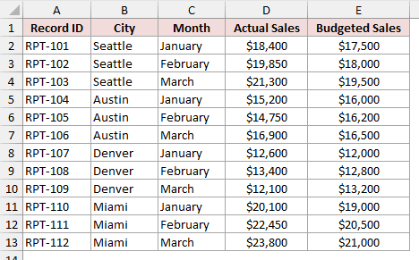
Below I have the Store Sales data in cells A1:E13, with one row per record and January, February, and March stored in the Month field.
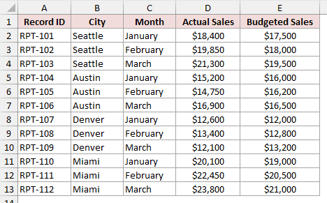
Here are the steps to compare each month’s Actual Sales with January:
- Create a PivotTable from
'Store Sales'!A1:E13, then place City in Rows, Month in Columns, and Actual Sales in Values.
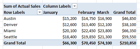
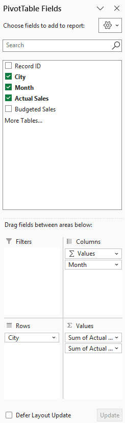
- Add Actual Sales to the Values area a second time. You need two copies: one keeps the sales values while the other shows the differences.
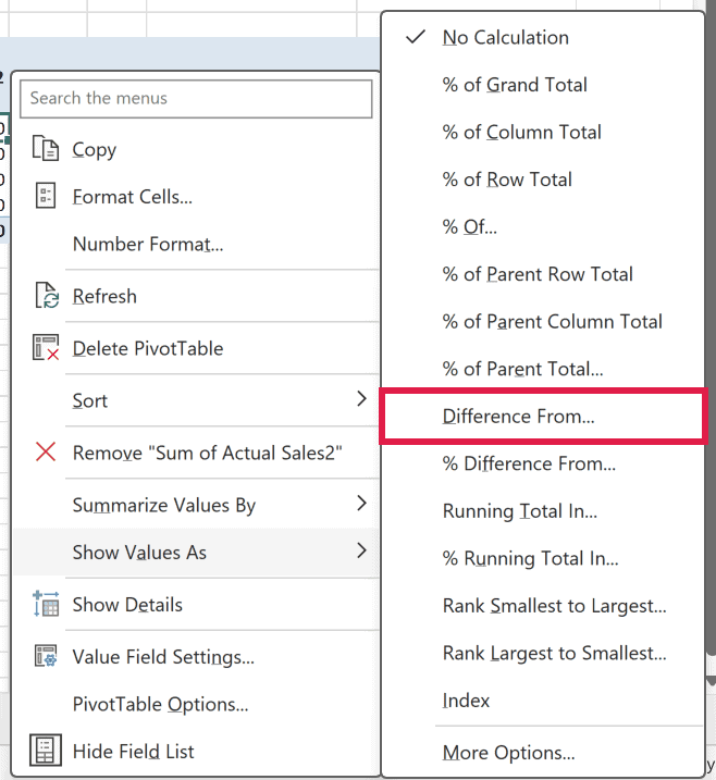
- Right-click a value in the second copy, then choose Show Values As > Difference From.
- Set the Base field to Month and the Base item to January, then confirm the settings.

You can now see how far each month’s Actual Sales sit above or below January without losing the original amounts.
Note: The Base field should not be the same field selected for the calculation. Here, Actual Sales is the value being calculated, so Month is the Base field.
Method #2: Using Show Values As % Difference From
Here’s the percentage version for the same-field scenario, where you care about the change relative to a base item instead of the dollar difference.
Below I have the same Store Sales range, A1:E13, and I want to compare February and March Actual Sales with January by city.
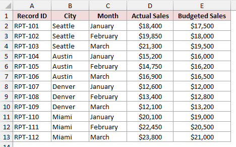
Here are the steps to show the percentage difference from January:
- Create a PivotTable from
'Store Sales'!A1:E13, then place City in Rows, Month in Columns, and Actual Sales in Values.
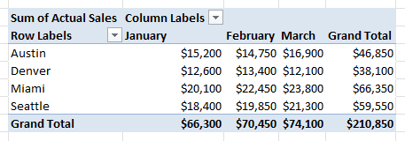
- Add Actual Sales to the Values area a second time so the PivotTable can keep both the sales amounts and the percentage differences.
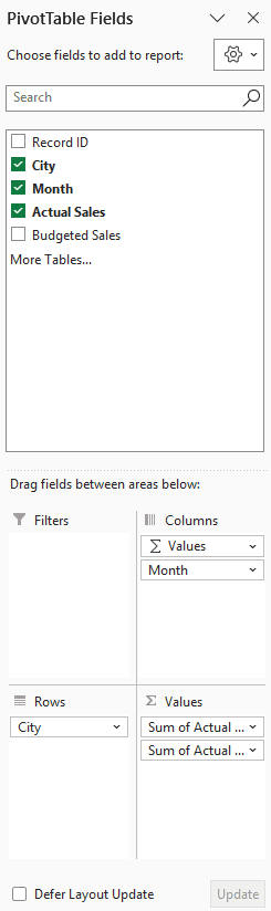
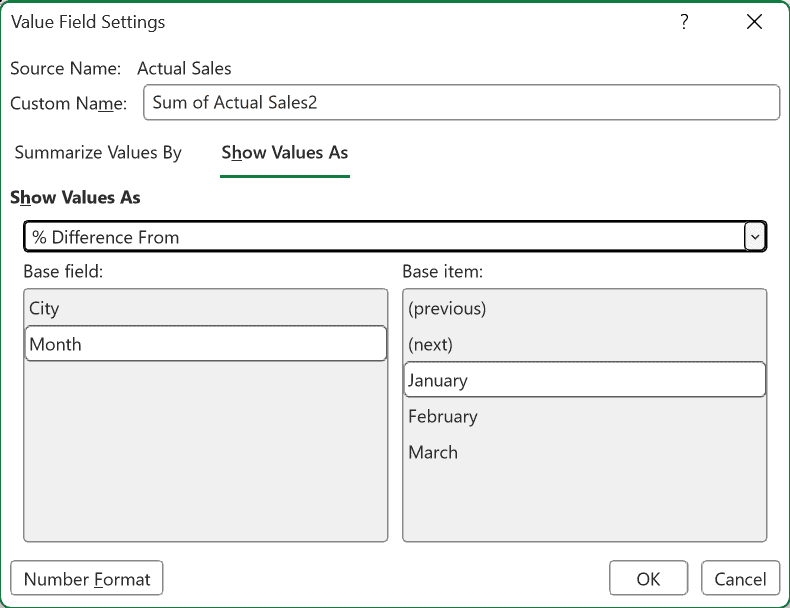
- Right-click a value in the second copy, then choose Show Values As > % Difference From.
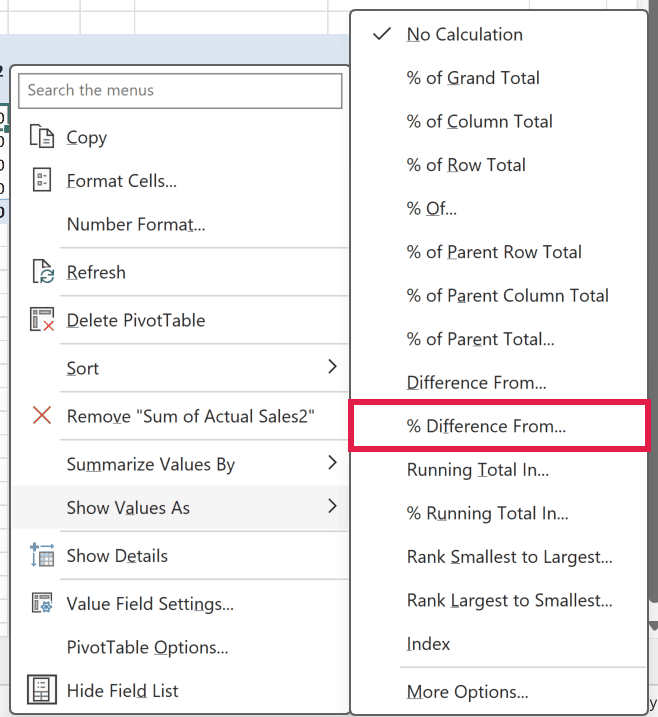
- Set the Base field to Month and the Base item to January, then confirm the settings.
Method #3: Using a Calculated Field
Show Values As stops working when the columns you want to compare come from different source fields.
For Actual Sales versus Budgeted Sales, you can use a calculated field to subtract one field from the other.
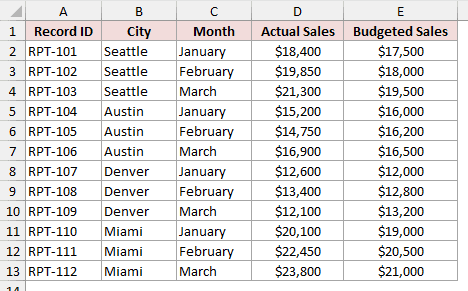
Below I have cells A1:E13 on the Store Sales sheet, where Actual Sales is in column D and Budgeted Sales is in column E.
Use this formula for the calculated field:
='Actual Sales'-'Budgeted Sales'
Here are the steps to add the difference to the PivotTable:
- Create a PivotTable from
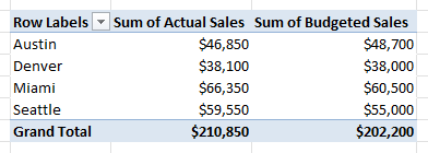
'Store Sales'!A1:E13, place City in Rows, and add Actual Sales and Budgeted Sales to Values.
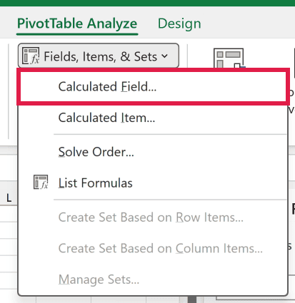
- Open PivotTable Analyze > Calculations > Fields, Items, & Sets > Calculated Field.
- Name the calculated field Sales Difference and enter the formula shown above.
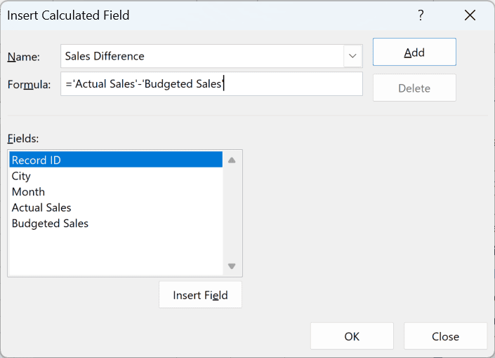
- Confirm the dialog to add Sales Difference to the PivotTable.
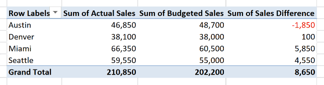
Note: Calculated fields work with the sums of the underlying data. Their formulas cannot use cell references, defined names, array functions, or PivotTable totals.
Method #4: Using a Calculated Item
If you want the difference to appear as another item inside the Month field, use a calculated item instead of a calculated field.
Below I have cells A1:E13 on the Store Sales sheet, with City in the PivotTable rows, Month in the columns, and Actual Sales in Values.
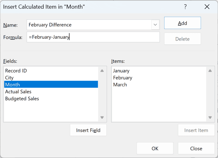
This formula creates a new Month item for February minus January:
=February-January
If the Month field is grouped, ungroup it first. Excel won’t add a calculated item to a grouped field.
Select the field, then choose PivotTable Analyze > Group > Ungroup.
Here are the steps to add the calculated item:
- Create a PivotTable from
'Store Sales'!A1:E13, then place City in Rows, Month in Columns, and Actual Sales in Values.
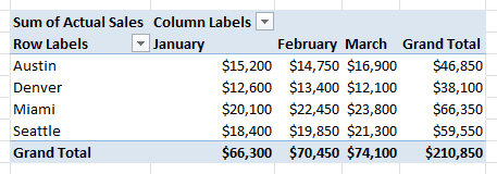
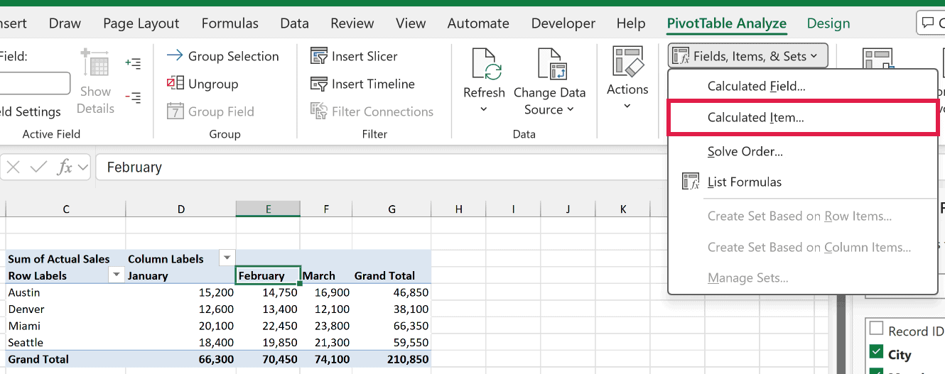
- Select the February heading in the PivotTable, then open PivotTable Analyze > Calculations > Fields, Items, & Sets > Calculated Item.
- Name the item February Difference and enter the formula shown above.
- Confirm the dialog to add the new item to the Month field.
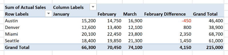
Note: A calculated item is added to the field itself, so Excel includes it in the subtotals and the Grand Total. Turn the Grand Total off for that field if the inflated number is confusing.
Method #5: Using a Measure in the Data Model
If your PivotTable uses the Data Model or Power Pivot, use a measure for the difference between Actual Sales and Budgeted Sales.
Calculated fields are unavailable in this setup. The measure performs the subtraction inside the model.
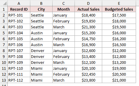
Below I have cells A1:E13 on the Store Sales sheet, with Actual Sales and Budgeted Sales stored as separate fields for each city and month.
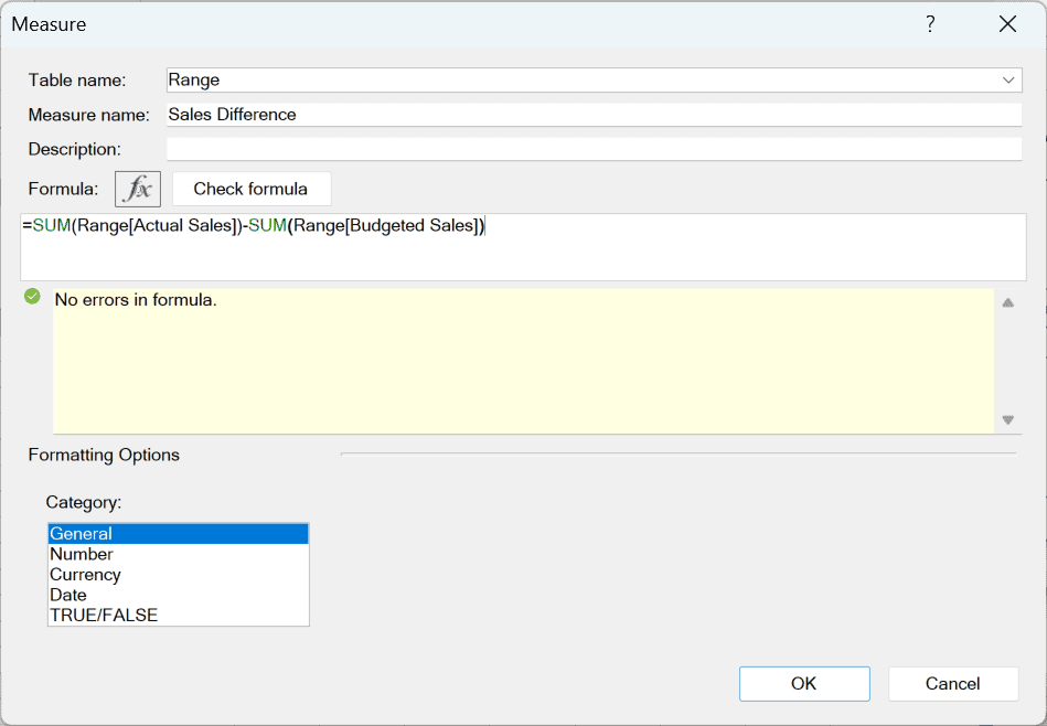
Excel names the table Range when this source range is added to the Data Model. Use this formula for the Sales Difference measure:
=SUM(Range[Actual Sales])-SUM(Range[Budgeted Sales])
Here are the steps to create and use the measure:
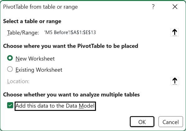
- Add the data in
'Store Sales'!A1:E13to the Data Model and create a PivotTable from that model.
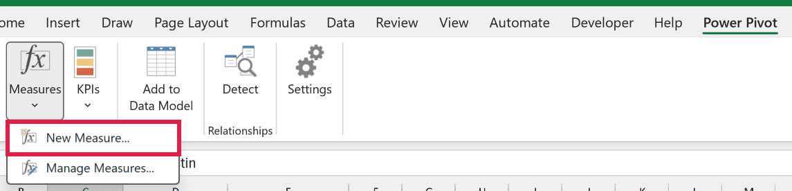
- On the Power Pivot tab, open Measures > New Measure.
- Name the measure Sales Difference. In the Formula box, subtract the SUM of Budgeted Sales from the SUM of Actual Sales.
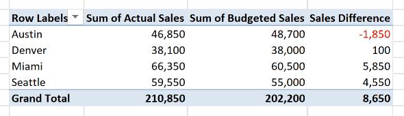
- Place City in Rows, then add Actual Sales, Budgeted Sales, and Sales Difference to Values.
Note: Power Pivot and the Data Model are Excel for Windows features, so this method isn’t available in Excel for Mac or Excel for the web. On a Mac, use the calculated field in Method #3 instead. On Windows, if you don’t see the Power Pivot tab, go to File > Options > Add-Ins, pick Disabled Items in the Manage box, select Go, then enable Microsoft Office Power Pivot.
Additional Notes About Showing the Difference Between Two Columns in a Pivot Table
- When the base value is small, check the dollar difference beside the percentage. A modest dollar change can look large as a percentage.
- Use a calculated item only when you want the result inside the existing column field. Use a calculated field or measure for the Values area.
- Excel for Mac’s Show Values As menu doesn’t list all the same options as Excel for Windows. Choose More Options on that menu to reach the one you want.
Frequently Asked Questions
Why Doesn’t the First Difference From Column Show a Difference?
The first month is the selected Base item, so Excel compares that month with itself.
Excel leaves the difference cells blank for the selected Base item. Here, that is January.
Can I Show the Difference Between Two Separate Columns Without a Calculated Field?
Show Values As only compares items within one source field, so it cannot subtract Actual Sales from Budgeted Sales.
Use a measure when the PivotTable uses the Data Model. Otherwise, use a calculated field for Actual Sales minus Budgeted Sales.
Can I Switch From a Dollar Difference to a Percentage?
Yes. On the second copy of the value field, change Show Values As from Difference From to % Difference From.
Keep the same Base field and Base item.
Why Is Calculated Field Greyed Out in My PivotTable?
Calculated fields are unavailable in an OLAP-connected PivotTable.
If the PivotTable uses the Data Model or Power Pivot, create a measure instead.
Can I Compare Cities Instead of Months?
Yes. Put City in Columns, then set the Base field to City and choose one city as the Base item.
Excel compares the other cities with that city.
Conclusion
I covered five ways to show a difference in a PivotTable. For columns that are items in one field, I reach for Show Values As Difference From first.
It keeps the original values visible and needs no formula. I hope you found this article helpful.
Other Excel articles you may also like:
