How to Show Percentage of Total in Pivot Table (5 Easy Ways)

Percentage of total in an Excel PivotTable shows you each item’s share of the whole, so you can spot which store or product contributes most.

With built-in Show Values As options, you don’t need formulas or an extra helper column.

I’ll show you grand and column totals, then compare shares within each store using row and parent totals.

You’ll also learn a DAX measure, a formula you add to the PivotTable’s Data Model to keep percentages fixed when filtering.

Table of Contents

Method #1: Using % of Grand Total

I’d start here for most comparisons. You can see each store’s share of all sales beside its dollar amount.

Show Values As is a setting on a value field. It changes how you see the numbers without touching your source data.

Below I have bakery sales with Sale ID, Store, Category, and Sales. I want each store’s share beside its sales amount.

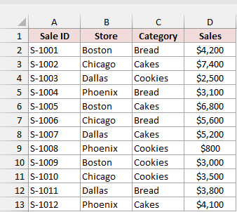
Bakery sales table with 12 rows and columns for Sale ID, Store, Category, and Sales.

I’ll use these steps to show each store’s percentage of total:

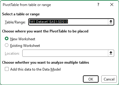
Select any cell in the dataset, go to the Insert tab, and click PivotTable. In the “PivotTable from table or range” dialog, keep New Worksheet selected and click OK.

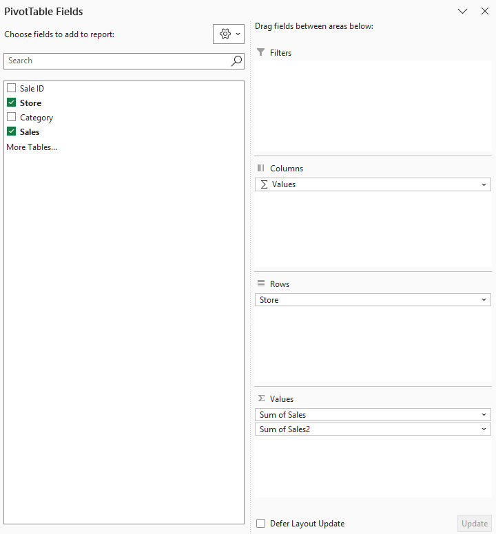
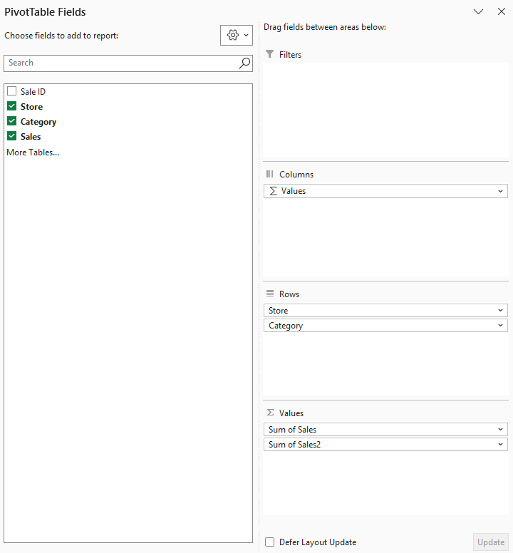
PivotTable creation dialog uses cells A1:D13 from M1 Dataset, with New Worksheet selected.

In the PivotTable Fields pane, check Store so it lands in Rows. Then drag Sales into Values twice. You’ll have two value columns, Sum of Sales and Sum of Sales2.

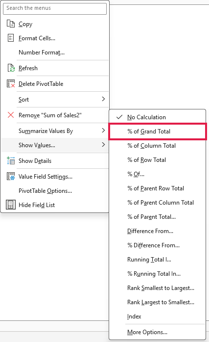
PivotTable Fields pane places Store in Rows and Sum of Sales and Sum of Sales2 in Values.

Right-click any number in the Sum of Sales2 column, go to Show Values As, and click % of Grand Total.

Show Values flyout for Sum of Sales2 highlights the % of Grand Total option in red.

Click the Sum of Sales2 header cell, type % of Total, and press Enter.

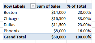
PivotTable lists sales and percentage of total by store, with Grand Total at 100.00%.

You’ll see these sales amounts and percentages:

Boston: $14,000 / 28.00%
Chicago: $16,500 / 33.00%
Dallas: $11,500 / 23.00%
Phoenix: $8,000 / 16.00%
Grand Total: $50,000 / 100.00%

Boston’s 28% comes from dividing $14,000 by the $50,000 grand total.

I added Sales twice so you can keep dollar amounts in one column and percentages in the other. If you only want percentages, add Sales once.

Excel won’t let you reuse “Sales” as the header because it’s already a field name. A name like “% of Total” works instead.

Note: You get two decimal places by default. To change them, right-click a percentage, choose Number Format, select Percentage, and set the decimal places.

Method #2: Using % of Column Total

For a category-by-category comparison, you can use % of Column Total.

Below I have bakery sales with Sale ID, Store, Category, and Sales. I want each store’s share of sales within each category.

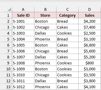
Bakery sales data lists Sale ID, Store, Category, and Sales for Boston, Chicago, Dallas, and Phoenix.

Follow Method #1 to create your PivotTable, adding Sales to Values only once. Put Store in Rows and Category in Columns.

PivotTable displays dollar sales by store, with Bread, Cakes, and Cookies arranged in columns.

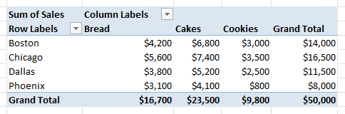
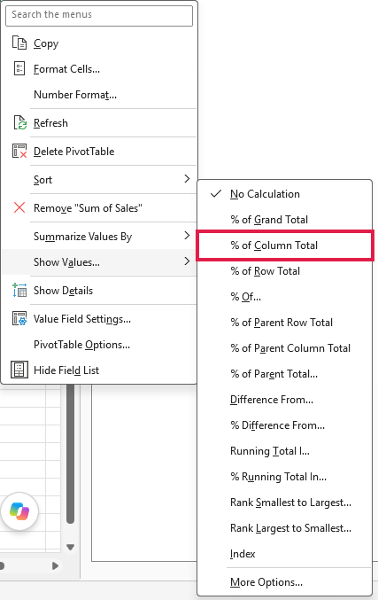
Here’s the step to change those dollar amounts to percentages:

Right-click any number in the PivotTable, go to Show Values As, and click % of Column Total.

Show Values flyout has the % of Column Total option outlined in a box.

Excel converts every number to a percentage of its column total.

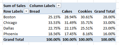
PivotTable shows store sales as percentages of each category column, with every column totaling 100%.

Read each row across Bread, Cakes, Cookies, and Grand Total, in that order:

Boston: 25.15%, 28.94%, 30.61%, 28.00%
Chicago: 33.53%, 31.49%, 35.71%, 33.00%
Dallas: 22.75%, 22.13%, 25.51%, 23.00%
Phoenix: 18.56%, 17.45%, 8.16%, 16.00%
Grand Total: 100.00% in every column

Within each column, the store shares add up to 100%, allowing for rounding in the percentages you see.

Boston’s 25.15% under Bread comes from $4,200 out of $16,700 in total Bread sales.

Phoenix’s smaller contribution to Cookies stands out at 8.16%. That’s $800 out of $9,800 in total Cookies sales.

In the Grand Total column, you can see each store’s share of all sales, matching the percentages from Method #1.

Method #3: Using % of Row Total

This time, you’ll look at each store’s product mix with % of Row Total.

Below I have bakery sales with Sale ID, Store, Category, and Sales. I want to see each store’s own product mix.

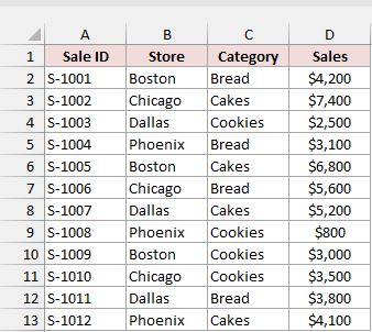
Excel grid contains 12 bakery sales records across four stores and the Bread, Cakes, and Cookies categories.

As in Method #2, put Store in Rows and Category in Columns. Add Sales to Values once to start with dollar amounts.

Sales PivotTable has stores down the rows and bakery categories across columns, with dollar amounts.

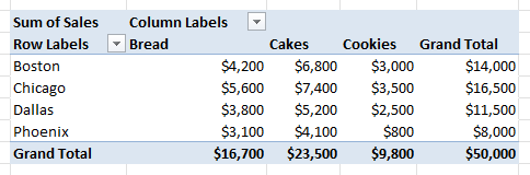
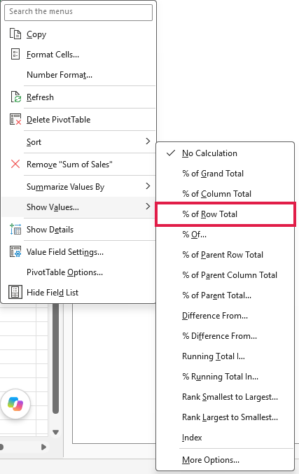
Here’s the step to show percentages within each store:

Right-click any number in the PivotTable, go to Show Values As, and click % of Row Total.

Show Values menu displays the % of Row Total option inside a highlighted box.

Now you can compare each category’s share of the total for its row.

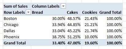
PivotTable displays category sales as percentages of each store row, with every row totaling 100%.

Read each row across Bread, Cakes, Cookies, and Grand Total, in that order:

Boston: 30.00%, 48.57%, 21.43%, 100.00%
Chicago: 33.94%, 44.85%, 21.21%, 100.00%
Dallas: 33.04%, 45.22%, 21.74%, 100.00%
Phoenix: 38.75%, 51.25%, 10.00%, 100.00%
Grand Total: 33.40%, 47.00%, 19.60%, 100.00%

Across each store’s row, the shares add up to 100% because you’re dividing its category sales by its own total.

Cakes bring in roughly half of every store’s sales. In Phoenix, they account for 51.25%.

In the Grand Total row, you can check the whole chain’s product mix. Cakes account for 47.00% of sales across all stores.

With column total, you’re comparing stores for each product. With row total, you’re comparing products within each store.

Method #4: Using % of Parent Row Total

For store and category comparisons in one nested PivotTable, I’d use % of Parent Row Total.

Below I have bakery sales with Sale ID, Store, Category, and Sales. I want category shares within stores and store shares overall.

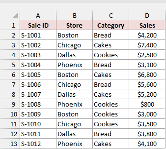
Bakery sales worksheet lists 12 records with sale identifiers, store names, categories, and sales amounts.

I’ll use these steps to put each category beneath its store:

Create a PivotTable as in Method #1. Check Store and then Category so both land in Rows, with Store above Category. Drag Sales into Values twice.

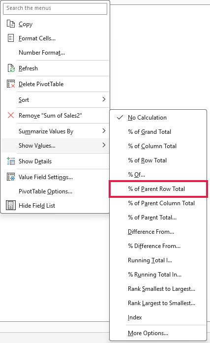
PivotTable Fields pane shows Store and Category in Rows, with two Sales fields in Values.

Right-click any number in the Sum of Sales2 column, go to Show Values As, and click % of Parent Row Total.

Show Values flyout highlights the % of Parent Row Total option with a box.

Click the Sum of Sales2 header cell, type % of Store Total, and press Enter.

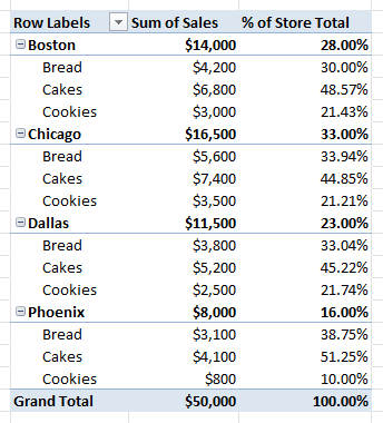
Nested PivotTable shows category sales and percentages beneath each store, with Boston Cakes at 48.57%.

You’ll see the following amounts under Sum of Sales and percentages under % of Store Total:

Boston: $14,000 / 28.00%

– Bread: $4,200 / 30.00% – Cakes: $6,800 / 48.57% – Cookies: $3,000 / 21.43%

Chicago: $16,500 / 33.00%

– Bread: $5,600 / 33.94% – Cakes: $7,400 / 44.85% – Cookies: $3,500 / 21.21%

Dallas: $11,500 / 23.00%

– Bread: $3,800 / 33.04% – Cakes: $5,200 / 45.22% – Cookies: $2,500 / 21.74%

Phoenix: $8,000 / 16.00%

– Bread: $3,100 / 38.75% – Cakes: $4,100 / 51.25% – Cookies: $800 / 10.00%

Grand Total: $50,000 / 100.00%

The store above a category is its “parent.” For Boston’s Cakes, you divide $6,800 by Boston’s $14,000 to get 48.57%.

Add the category percentages beneath each store and you’ll get 100%, allowing for rounding.

For the store rows, you’re comparing each store with its parent, the grand total. Boston shows 28%, Chicago 33%, Dallas 23%, and Phoenix 16%.

Method #5: Using a DAX Measure (Data Model)

If you need to keep dividing by the full dataset total as you filter, I’d use a DAX measure.

With Show Values As, you divide by what’s visible in the PivotTable. If you hide a store, you’ll see the remaining shares increase to fill 100%.

You can use the Data Model, a workbook data store, for PivotTables, and write its measures in the DAX formula language.

Below I have bakery sales with Sale ID, Store, Category, and Sales in a table named SalesData. I want percentages based on the full dataset.

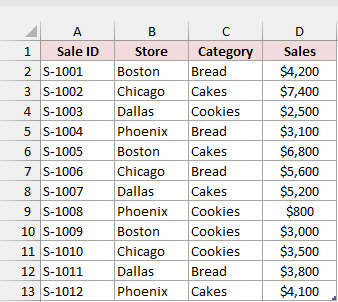
Bakery sales data appears in an Excel Table named SalesData, with four columns and 12 records.

If you haven’t made a Table yet, select any cell, press Ctrl + T, and click OK. Type SalesData in Table Design’s Table Name box.

I’ll use these steps to create the measure:

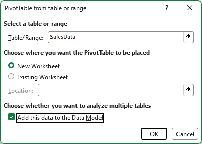
Select any cell in the table, go to the Insert tab, and click PivotTable. In the dialog, check “Add this data to the Data Model” and click OK.

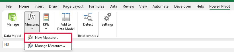
PivotTable dialog uses SalesData as its source, with Add this data to the Data Model checked.

Go to the Power Pivot tab, click Measures, and then click New Measure.

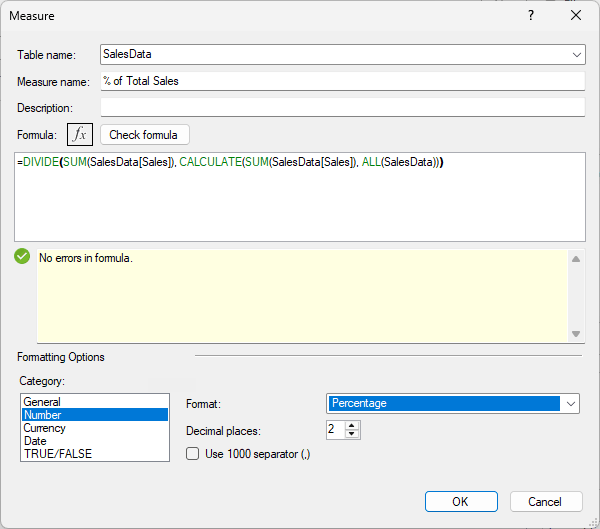
Power Pivot tab shows the Measures dropdown open, with New Measure outlined in a box.

In the Measure dialog, keep SalesData as the Table name and type % of Total Sales as the Measure name.
Type the formula below in the Formula box after its existing equals sign. Don’t add a second equals sign.

=DIVIDE(SUM(SalesData[Sales]), CALCULATE(SUM(SalesData[Sales]), ALL(SalesData)))

Under Formatting Options, pick Number as the Category and Percentage as the Format, then click OK.

Measure dialog shows % of Total Sales using DIVIDE, CALCULATE, and ALL, formatted as percentages with two decimals.

In the PivotTable Fields pane, check Store for Rows, Sales for Values, and the new % of Total Sales measure for Values.

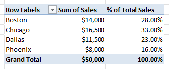
PivotTable displays sales and the % of Total Sales measure by store, with Grand Total at 100.00%.

You’ll see the sales amount beside % of Total Sales:

Boston: $14,000 / 28.00%
Chicago: $16,500 / 33.00%
Dallas: $11,500 / 23.00%
Phoenix: $8,000 / 16.00%
Grand Total: $50,000 / 100.00%

How does this formula work?

First, SUM(SalesData[Sales]) adds up sales for the current PivotTable row. On Boston’s row, I’m adding Boston’s sales.

For the denominator, I remove every filter on SalesData with CALCULATE(SUM(SalesData[Sales]), ALL(SalesData)). That always returns the full $50,000.

Finally, DIVIDE divides the current row’s sales by that total. If the total is ever zero, you get a blank instead of an error.

You can reuse this measure in any PivotTable built on the same Data Model.

If you filter Store to hide Phoenix, you’ll still see these percentages:

Boston: 28.00%
Chicago: 33.00%
Dallas: 23.00%
Grand Total: 84.00%

That 84.00% is the visible stores’ share of all sales. You’re still dividing their $42,000 by the full $50,000.

With Show Values As instead, you’d see Boston at 33.33%, Chicago at 39.29%, and Dallas at 27.38%, because you’d be dividing by $42,000.

Note: If you don’t have a Power Pivot tab, right-click SalesData in the PivotTable Fields pane and choose Add Measure. You’ll open the same dialog.

For this method, you’ll need Excel 2016 or later for Windows, including Microsoft 365. Excel for Mac doesn’t support Data Model measures.

Additional Notes About Showing Percentage of Total in a Pivot Table

Show Values As percentages follow your filters and slicers. If you hide a store, the remaining shares add up to 100% again. Use Method #5 to keep original shares.
These settings change how you see the numbers without touching your source data. To restore amounts, right-click a value and choose Show Values As, then No Calculation.
After changing source data, you’ll need to refresh the PivotTable. Go to PivotTable Analyze and click Refresh so your percentages update too.
For other percentage comparisons, you can choose these Show Values As options:

– With nested Columns, % of Parent Column Total lets you make the same comparison as Method #4. – If you want to choose the parent field yourself, use % of Parent Total. – For a comparison with one base item you choose, rather than a total, use % Of.

Frequently Asked Questions

I’ll answer why you might see 100% in every row, how totals differ, and how to show percentages beside amounts without a calculated field.

Why Does My Pivot Table Show 100% in Every Row?

If you use % of Row Total with Store in Rows and nothing in Columns, you’ll get 100.00% on every row.

You’re comparing each row’s only value with itself. Use % of Grand Total or % of Column Total to compare stores instead.

What’s the Difference Between % of Grand Total and % of Column Total?

With nothing in Columns, you’ll get the same store percentages with either option: 28%, 33%, 23%, and 16%.

With a field in Columns, you divide by each column’s total using % of Column Total. With % of Grand Total, you divide by the overall total.

Can I Use a Calculated Field to Get Percentage of Total?

You can use a calculated field to work on the summed values for each cell of the PivotTable, but you can’t reference the grand total or any other total.

Use Show Values As or create a DAX measure as in Method #5.

How Do I Show the Amount and the Percentage Side by Side?

Add the same value field to Values twice. Apply Show Values As to one copy and keep the other as the amount, as in Method #1.

Conclusion

I’d start with % of Grand Total for most comparisons. You can see each item’s share of the whole beside its amount with a few clicks.

I hope you found this article helpful.

Other Excel articles you may also like:

How to Show Percentage of Total in an Excel Pivot Table