How to Add a Calculated Item to a Pivot Table in Excel

A calculated item adds a new row or column inside an Excel PivotTable field, so you can combine or compare existing items without changing your source data.

For example, you can add an Accessories row that combines Keyboard and Mouse, or a Change column that subtracts last year’s sales from this year’s.

You do need to watch the totals, because Excel includes the new item alongside the items used in its formula.

I’ll show you how to combine product sales, calculate the change between years, and fix the grand totals in both examples.

What Is a Calculated Item in a Pivot Table?

Suppose your PivotTable lists Keyboard and Mouse separately, but you want an Accessories row that adds their sales. You can create that row with a calculated item.

A calculated item sits inside an existing row or column field. Its formula uses other items from that same field, such as Keyboard and Mouse from Product.

It works on their summed values. Each cell in the new item uses the matching cells of the items in its formula.

A calculated field adds a new value column using source columns, such as Sales minus Cost. A calculated item combines or compares items within one field.

How to Add a Calculated Item to a Pivot Table

I’ll combine Keyboard and Mouse sales into an Accessories row, keeping the source data as it is.

Below I have a dataset containing 16 sales orders with the region, product, year, and sales amount.

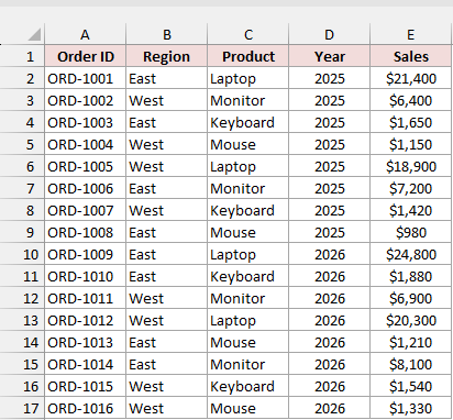
On the Sales Data sheet, the Excel Table named SalesData occupies A1:E17. The orders cover the East and West regions in 2025 and 2026.

I’ve set up a PivotTable with Product in Rows and Sum of Sales in Values.

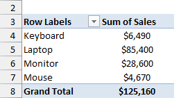
It shows these sales amounts before I add anything:

• Keyboard: $6,490
• Laptop: $85,400
• Monitor: $28,600
• Mouse: $4,670
• Grand Total: $125,160

Here are the steps to add the Accessories row:

1. Click any product name in the PivotTable, such as Keyboard.

Select an item label in the Rows or Columns area. If you select a value cell instead, the Calculated Item command stays greyed out.

2. Go to the PivotTable Analyze tab, click Fields, Items, & Sets in the Calculations group, then click Calculated Item.

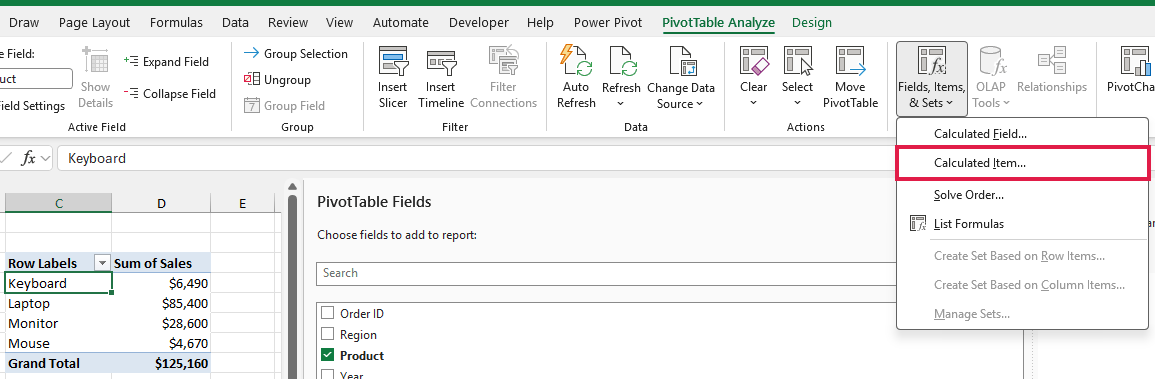
3. In the Insert Calculated Item dialog, type Accessories in the Name box. In the Formula box, delete = 0 and enter the formula below.

=Keyboard+Mouse

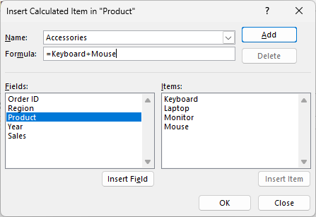
The dialog title reads Insert Calculated Item in "Product", so you can check that you’re adding an item to the right field.

You can also select Keyboard in the Items list and click Insert Item, type +, then insert Mouse.

4. Click Add, then click OK.

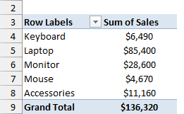
The new Accessories row appears at the bottom of the product list. It shows $11,160, which is $6,490 plus $4,670.

The Grand Total has also increased to $136,320. I’ll fix that next. You can find the finished example on the Combine Items sheet.

How to Fix the Grand Total After Adding a Calculated Item

The Grand Total adds every visible row. Keyboard and Mouse now count twice: once in their own rows and again in Accessories.

The difference is $136,320 minus $125,160, or $11,160. That’s exactly the amount in the Accessories row.

To use Accessories in place of its two products, hide Keyboard and Mouse with the field’s filter.

Here are the steps to correct the total:

1. Click the filter arrow on the Row Labels heading.
2. Uncheck Keyboard and Mouse.
3. Click OK.

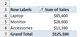
You now have these rows:

• Laptop: $85,400
• Monitor: $28,600
• Accessories: $11,160
• Grand Total: $125,160

The Grand Total matches the source data again. Accessories still calculates correctly even though you’ve hidden Keyboard and Mouse.

How to Add a Calculated Item to a Column Field

You can also compare items across columns. I’ll add a Change column that subtracts each product’s 2025 sales from its 2026 sales.

For this example, I have 16 sales orders with the region, product, year, and sales amount.

The starting PivotTable has Product in Rows, Year in Columns, and Sum of Sales in Values.

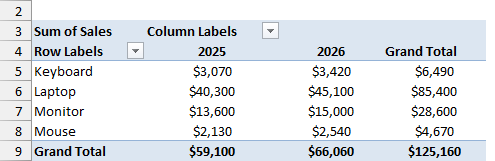
Here are the steps to add the Change column:

1. Click a year heading in the PivotTable, such as 2025.
2. Go to the PivotTable Analyze tab, click Fields, Items, & Sets, then click Calculated Item.
3. Type Change in the Name box. Replace the contents of the Formula box with the formula below.

='2026'-'2025'

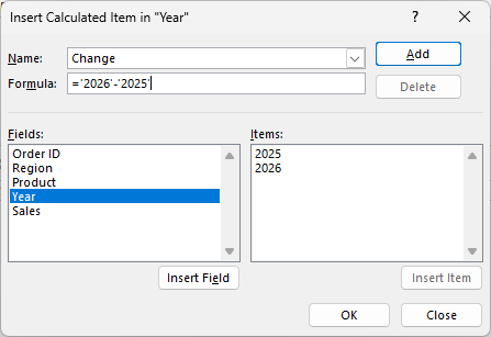
This time, the dialog title reads Insert Calculated Item in "Year".

Note: Wrap numeric item names in single quotes. Without them, Excel reads 2026 and 2025 as plain numbers, so =2026-2025 returns 1 in every row instead of the sales difference. Use single quotes around item names that have more than one word or contain numbers or symbols.

4. Click Add, then click OK.

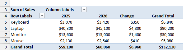
The Change column shows the increase for each product:

• Keyboard: $350
• Laptop: $4,800
• Monitor: $1,400
• Mouse: $410
• Grand Total: $6,960

The right-hand Grand Total column now adds 2025, 2026, and Change. For Keyboard, it shows $6,840 instead of the actual sales total of $6,490.

That column mixes sales with the difference between years. I’ll turn it off while keeping the Grand Total row at the bottom.

Here is the step to remove the Grand Total column:

1. On the Design tab, click Grand Totals, then click On for Columns Only.

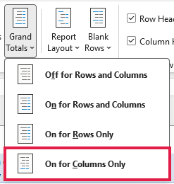
The right-hand Grand Total column disappears, while the Grand Total row stays at the bottom.

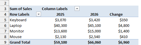
The bottom row still shows the $6,960 increase across all products. You can find this finished example on the Change Between Years sheet.

How to Edit or Delete a Calculated Item

You can change an existing calculated item’s formula without creating another item. Start by selecting an item in the field that contains it, such as a product name.

Here are the steps to edit it:

1. Go to PivotTable Analyze, click Fields, Items, & Sets, then click Calculated Item.
2. Pick the calculated item from the Name dropdown and change its formula.
3. Click Modify, then click OK.

Deleting an item removes it for good. If you only want it out of sight, hide it with the field’s filter instead.

To delete it, open the same dialog, pick the item in the Name dropdown, click Delete, then click OK.

How to See All Calculated Item Formulas

If you’ve inherited a workbook and can’t trace a PivotTable’s numbers, you can have Excel list its formulas on a new worksheet.

Here is the step to create the list:

1. Select the PivotTable, go to PivotTable Analyze, click Fields, Items, & Sets, then click List Formulas.

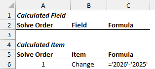
Excel adds a worksheet listing every calculated field and calculated item in that PivotTable, with its solve order, name, and formula.

For the year comparison, the Calculated Item section shows Solve Order 1, Item Change, and Formula ='2026'-'2025'.

The example workbook includes this output on the Formula List sheet.

Additional Notes About Calculated Items in Pivot Tables

Before you use a calculated item in another PivotTable, check these limits and how they affect your layout:

• You can’t add a calculated item to a grouped field. Excel shows: “This PivotTable report field is grouped. You cannot add a calculated item to a grouped field.” Ungroup first using PivotTable Analyze > Ungroup, add the item, then group again if you need to.
• A PivotTable with a calculated item can’t summarize values with Average, StdDev, or Var. Excel shows: “Averages, standard deviations, and variances are not supported when a PivotTable report has calculated items.” Sum works fine.
• You can’t add the same source field to Values twice while a calculated item exists. Excel shows: “Multiple data fields of the same field are not supported when a PivotTable report has calculated items.”
• Subtotals include calculated items too. With Region above Product in Rows, each region subtotal adds Accessories on top of Keyboard and Mouse. Hide the replaced items to avoid counting them twice.
• Calculated item formulas can’t use cell references or defined names, and they can’t refer to totals.
• Calculated items aren’t available for PivotTables built on the Data Model or an OLAP source. Use a measure there instead.

Frequently Asked Questions

These questions cover updating a calculated item and using it without changing the source data.

Can a Calculated Item Use a Value From a Worksheet Cell?

No, you can’t reference a worksheet cell. You can put the number directly in the formula, though. For example, this multiplies the 2026 item’s sales by 1.1:

='2026'*1.1

Does a Calculated Item Update When the Source Data Changes?

Yes, after you refresh the PivotTable. Excel recalculates the item using the refreshed values, so you don’t need to rewrite its formula when sales amounts change.

How Do I Hide a Calculated Item Without Deleting It?

Open the field’s filter, uncheck the calculated item’s name, then click OK. For Accessories, you would uncheck Accessories rather than Keyboard and Mouse.

Conclusion

To add a calculated item, select an item label, open Calculated Item from PivotTable Analyze, and enter a name and formula.

I recommend checking the grand totals afterward and using single quotes around numeric item names.

Use a calculated field when you need a formula based on source columns, or a measure when your PivotTable uses the Data Model or an OLAP source.

Other Excel articles you may also like:

• GETPIVOTDATA Function in Excel
• Pivot Table vs Pivot Chart in Excel
• PIVOTBY Function in Excel
• How to Group by Months in Excel Pivot Table?
• How to Use Slicers in Excel (Beginner to Advanced Guide)