How to Use a Timeline in a PivotTable in Excel

A Timeline in Excel is a date filter for PivotTables.

Instead of ticking dates in a drop-down, you drag across a bar of months, and the PivotTable shows only that period.

It makes questions like “what did we sell last quarter?” a one-click job. You can also switch the bar between years, quarters, months, and days.

The catch is that Timelines are picky. They only work with PivotTables, the date column has to hold real dates, and there’s no week level.

In this article, I’ll show you how to insert a Timeline, pick a date range, connect it to several PivotTables, filter by week, and fix a Timeline that isn’t working.

How to Insert a Timeline in a PivotTable

A Timeline sits next to your PivotTable and filters it by date. You need a PivotTable built from data that has a date column.

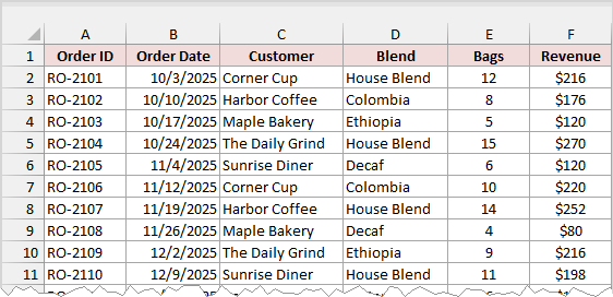
Below I have a dataset of 24 wholesale orders from a coffee roaster, placed between October 2025 and March 2026.

Each order has an order date, the customer, the coffee blend, the number of bags, and the revenue.

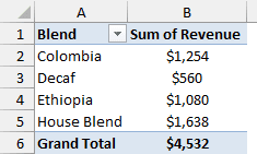
I’ve made a PivotTable from this data that shows the total revenue for each blend. The grand total is $4,532.

Now I want to filter this PivotTable by order date with a Timeline.

Here are the steps to insert a Timeline in a PivotTable:

1. Select any cell in the PivotTable.
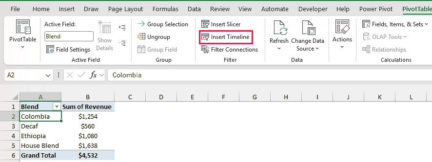
2. Go to the PivotTable Analyze tab and click Insert Timeline.

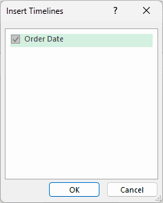
3. In the Insert Timelines dialog box, check Order Date and click OK.

Excel adds a Timeline for the Order Date field.

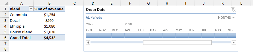
The label at the top says All Periods, which means nothing is filtered yet. Below it, there’s one tile for each month, with the year above.

The MONTHS drop-down on the right changes the time level, and the scrollbar at the bottom moves you through the months.

Note: Timelines need Excel 2013 or later on Windows. You can also insert one from the Insert tab by clicking Timeline while a cell in the PivotTable is selected.

Filtering a PivotTable by Month With a Timeline

Once the Timeline is in place, filtering is one click. I’m using the same revenue PivotTable, with the Timeline showing all periods.

To show a single month, click its tile. Here I’ve clicked JAN under 2026.

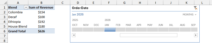
The label changes to Jan 2026, and the PivotTable shows only the four January orders. The grand total drops to $626.

If the month you want isn’t visible, drag the scrollbar at the bottom of the Timeline, or click the arrows at either end.

Picking a Date Range in a Timeline

A Timeline can filter any run of months in one go, like the last three months or a whole season.

Starting from the same PivotTable, I want the revenue from November 2025 to January 2026.

Click the NOV tile and drag across to JAN. You can also click NOV, hold Shift, and click JAN.

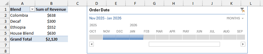
The label shows Nov 2025 – Jan 2026, and the grand total is now $2,120.

To make the range longer or shorter, drag the handle on either end of the highlighted bar.

Note: A Timeline filters one continuous range. You can’t pick November and January while skipping December.

Changing the Time Level (Years, Quarters, Months, Days)

A new Timeline shows months. You can switch it to years, quarters, or days, depending on how wide a period you want to filter.

To change the level, click the MONTHS drop-down in the top-right corner of the Timeline and pick a level.

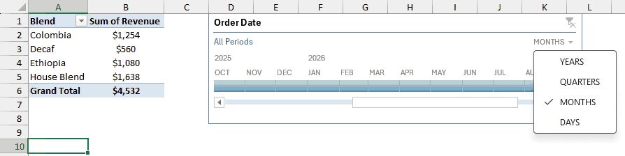
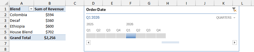
Here I’ve switched to QUARTERS and clicked Q1 under 2026. The PivotTable now shows only January to March 2026, with a grand total of $2,256.

The YEARS level gives you one tile per year, and DAYS gives you one tile per day. I use the Days level in the week section below.

If you already have a range selected, switching the level doesn’t reset it. The PivotTable keeps the same filter until you click a new tile.

Connecting One Timeline to Multiple PivotTables

One Timeline can filter several PivotTables at once. It works just like when you connect a slicer to multiple pivot tables, through Report Connections.

Here I have two PivotTables from the same coffee orders. The first one shows revenue by blend, and the second one shows bags by customer.

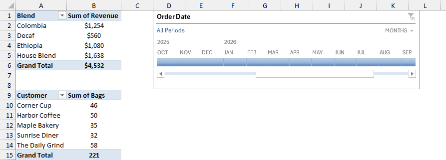
The Timeline is connected to the first PivotTable only, so the bags PivotTable ignores it.

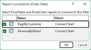
Here are the steps to connect the Timeline to the second PivotTable:

1. Select the Timeline, go to the Timeline tab, and click Report Connections. You can also right-click the Timeline and pick Report Connections.
2. Check the second PivotTable and click OK.

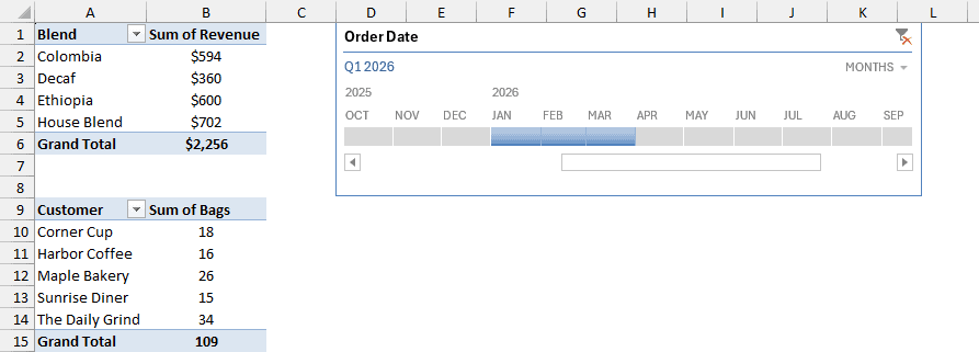
Now click Q1 2026 in the Timeline, or pick January to March. Both PivotTables filter together, and the bags PivotTable shows 109 bags for the quarter.

If the PivotTable you want isn’t in the Report Connections list, it doesn’t share the same PivotCache. That’s the stored copy of the source data Excel keeps for PivotTables.

A Timeline can only connect PivotTables that share one.

Formatting a Timeline

When you select a Timeline, Excel shows the Timeline tab. This is where you change how it looks.

These are the main options on the Timeline tab:

• Timeline Styles: pick a color scheme from the gallery.
• Show group: turn the Header, Selection Label, Scrollbar, and Time Level on or off.
• Size group: set the height and width of the Timeline.

Here I’ve picked a dark red style from the gallery and turned off the scrollbar. The Timeline still filters the PivotTable to Q1 2026.

Hiding the scrollbar and the time level is handy on a dashboard, where you want the Timeline to take up less space.

Clearing or Removing a Timeline

To clear the filter, click the Clear Filter button in the top-right corner of the Timeline. The label goes back to All Periods, and the PivotTable shows all orders again.

To remove the Timeline completely, click its border to select it and press Delete.

Deleting a Timeline also removes its filter, so the PivotTable goes back to $4,532. That’s different from a slicer, which leaves its filter in place when you delete it.

Filtering a Pivot Table Timeline by Week

A Timeline has no week level. It stops at years, quarters, months, and days, so you need a workaround to filter by week.

Here are three ways to do it, from quickest to most flexible.

Using the Days Level

This works when you need one week now and then. Switch the Timeline to DAYS, click the first day of the week, hold Shift, and click the last day.

Here I’ve picked Monday, January 5, to Sunday, January 11, 2026, on the same revenue PivotTable.

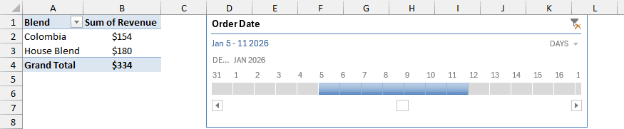
The label shows Jan 5 – 11 2026, and the PivotTable shows the two orders from that week, for a total of $334.

Grouping the Dates Into Weeks

If you want to see every week as its own row, group the dates in the PivotTable into 7-day weeks.

Here I have a PivotTable with Order Date in the Rows area and revenue in the Values area.

Here are the steps to group the dates into weeks:

1. Right-click any date in the PivotTable and click Group.
2. In the Grouping dialog box, set Starting at to a Monday, like 9/29/2025, and Ending at to a Sunday, like 3/29/2026.
3. Under By, select Days only, set Number of days to 7, and click OK.

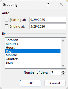
Each row is now one week, from Monday to Sunday. The Timeline still works on the grouped dates, so you can pick a month and see its weeks.

Here I’ve clicked JAN 2026 in the Timeline. The PivotTable shows three weeks, because nothing was ordered in the week of January 12.

Excel selects Months by default, so click it to unselect it. Excel only groups by a number of days when Days is the only option selected.

Using a Week Starting Column and a Slicer

If you’d rather click a button for each week, add a column with the start date of each week, then use a normal slicer on it.

Below I have the same coffee orders with a new Week Starting column. It uses this formula:

=B2-WEEKDAY(B2,3)

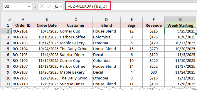
WEEKDAY with 3 as the second argument returns 0 for Monday, 1 for Tuesday, and so on up to 6 for Sunday.

Subtracting that number from the order date takes you back to the Monday of that week. Format the column as a date.

Now refresh the PivotTable, go to PivotTable Analyze > Insert Slicer, and check Week Starting.

Here I’ve clicked 1/5/2026 in the slicer. The PivotTable shows the same $334 as the Days level.

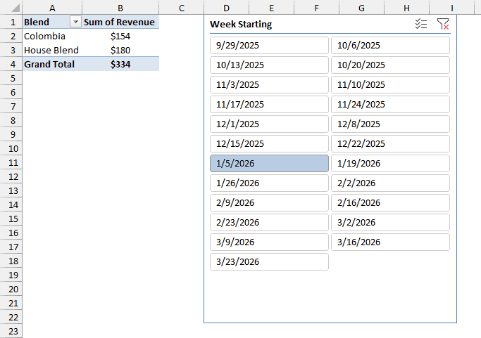
The slicer lists only the weeks that have orders, so there are no empty buttons to scroll past.

Timeline vs Date Slicer

A Timeline is a slicer built for dates. A normal slicer in Excel can filter a date field too, but it shows one button per date.

Here I’ve added a slicer for Order Date next to a Timeline. The slicer has 24 buttons, one for each order date.

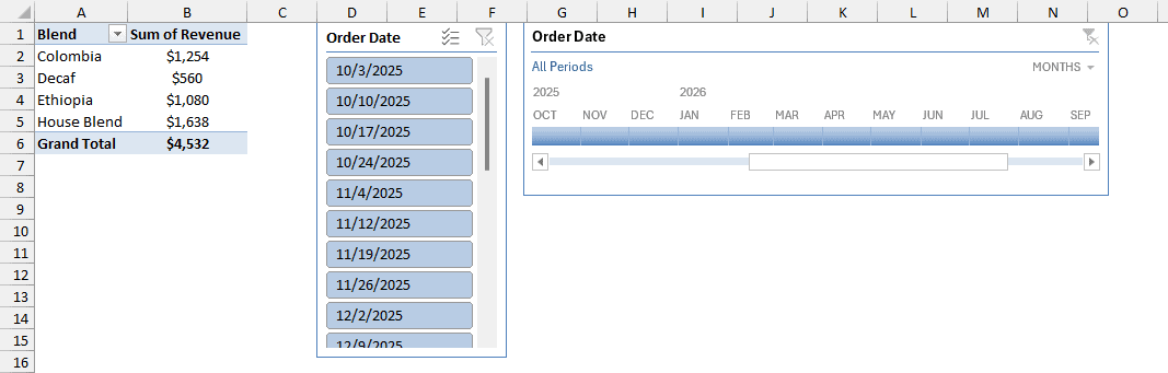
Here’s how the two compare:

	Timeline	Date slicer
Filters	Date fields only	Any field, including dates
What you click	A bar of periods	One button per date
Time levels	Years, quarters, months, days	None, only the exact dates
Picking a date range	Drag across the bar	Shift-click a run of buttons
Picking periods that aren’t next to each other	No	Yes, with Ctrl-click
Works with Excel Tables	No, PivotTables only	Yes

For dates, use a Timeline. Use a slicer when you need to pick separate dates, or when you’re filtering a Table instead of a PivotTable.

Pivot Table Timeline Not Working? Common Fixes

Most Timeline problems start in the data or the PivotTable. Here are the ones you’re most likely to run into.

Insert Timeline Is Greyed Out or Asks for a Connection

Check these first:

• The active cell is inside a PivotTable. The PivotTable Analyze tab only appears when a PivotTable cell is selected.
• You’re not starting from a normal range or an Excel Table. There, Insert > Timeline opens the Existing Connections dialog box instead, because a Timeline needs a PivotTable.
• The workbook isn’t in Compatibility Mode. In an .xls file, Insert Timeline is greyed out, so save the file as .xlsx and reopen it.
• You’re on Excel 2013 or later. Older versions don’t have Timelines.

The “Field Not Formatted as Date” Error

Excel shows this error when the PivotTable has no field with real dates in it. The dates look fine, but Excel stores them as text.

Even one text entry in the date column, like TBD, is enough to trigger it. Blank cells are fine.

Below I have six coffee orders where the order dates were typed as text, like 10/03/2025.

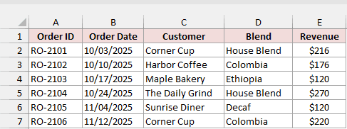
When I try to insert a Timeline for this PivotTable, Excel says: “We can’t create a Timeline for this report because it doesn’t have a field formatted as Date.”

To check whether a date is real, use ISNUMBER on it. Excel stores real dates as numbers, so ISNUMBER returns TRUE for them and FALSE for text.

=ISNUMBER(B2)

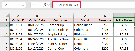
Every row returns FALSE here, so these dates are text.

Here are the steps to convert the text to real dates with Text to Columns:

1. Select the dates in the Order Date column.
2. Go to the Data tab and click Text to Columns.
3. Click Finish without changing anything.
4. Right-click the PivotTable and click Refresh.

The ISNUMBER column now shows TRUE, and Insert Timeline works on the refreshed PivotTable.

Note: Text to Columns reads the dates using your computer’s date settings. If your text dates put the day first, click Next twice instead, choose Date, and pick DMY.

New Dates Don’t Show Up in the Timeline

A Timeline only knows about the dates in the PivotTable’s cache. When you add orders for a new month, the Timeline won’t filter them until you refresh the PivotTable.

Right-click the PivotTable and click Refresh, or press Alt + F5.

The Timeline Doesn’t Filter Another PivotTable

Each Timeline filters only the PivotTables it’s connected to. Select it, go to Timeline > Report Connections, and check the PivotTable you want.

If the PivotTable isn’t in the list, it doesn’t share the Timeline’s PivotCache, so the Timeline can’t reach it.

The Timeline Clears a Date Slicer’s Selection

By default, a PivotTable allows only one filter per field. A Timeline and a slicer on the same date field then cancel each other out.

To use both together, right-click the PivotTable, click PivotTable Options, and check Allow multiple filters per field on the Totals & Filters tab.

Additional Notes About Using a Timeline in Excel

• Build your PivotTable from an Excel Table. New rows added to the Table flow into the PivotTable when you refresh it, so the Timeline never misses a month.
• A Timeline spans whole calendar years. If your data runs from October to March, you’ll still see tiles for the empty months at either end.
• In the example file, the Timeline Report sheet has one Timeline connected to both PivotTables, and the Weekly Report and Week Slicer sheets show the week workarounds.

Frequently Asked Questions

Here are answers to a few more questions about Timelines.

Can I use a Timeline without a PivotTable?

No. Timelines only work with PivotTables. If your data is in an Excel Table, create a PivotTable from it first, or use a normal slicer on the Table.

Can a slicer filter dates by month?

Yes, if you group the date field by month first. Right-click a date in the PivotTable, click Group, and select Months and Years.

Excel adds a Months field and a Years field, and you can insert a slicer for each. You need both, because a Jan button covers January of every year.

Why can’t I select January and March without February?

A Timeline filters one continuous range only.

To pick months that aren’t next to each other, group the dates by month and use a slicer, then Ctrl-click the months you want.

Conclusion

A Timeline is the easiest way to filter a PivotTable by date.

I showed you how to insert one, pick a range, change the time level, and connect it to more than one PivotTable.

I also covered three ways to filter by week and how to fix a Timeline that won’t work. I hope you found this article helpful.

Other Excel articles you may also like:

• How to Group by Quarters in Excel Pivot Table?
• Slicer vs Filter in Excel
• Insert Slicer Greyed Out in Excel