Connect Slicer to Multiple Pivot Tables (Step-by-Step)

When you have two or more PivotTables built from the same data, you usually want them to filter together.

Click one slicer button, and every report on the sheet changes at once.

Excel can do this with a single slicer. The catch is that the PivotTables must share a data source, which isn’t obvious when one refuses to connect.

In this article, I’ll show you how to connect one slicer to several PivotTables, link PivotTables from different data sources, and fix one that won’t connect.

Table of Contents

Connect Slicer to Multiple Pivot Tables (Same Data Source)

This is the most common setup. You build a few PivotTables from one dataset to look at it from different angles, and one slicer filters all of them.

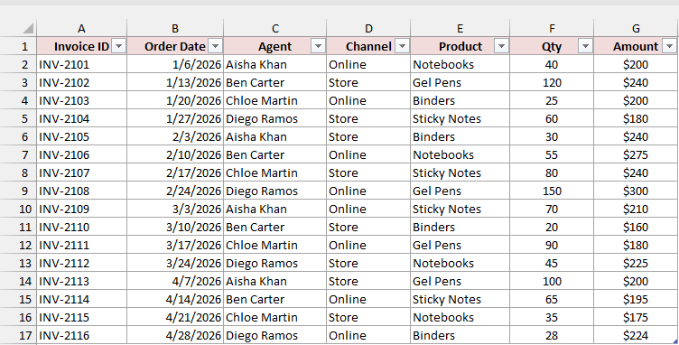
Below I have the sales data for a stationery company. It’s an Excel Table named Sales, with 16 orders from four sales agents.

Sales Table with invoice, date, agent, channel, product, qty, and amount

I’ve made two PivotTables from this Table. The first shows sales by product and the second shows sales by channel (Online or Store). Both totals are $3,444.

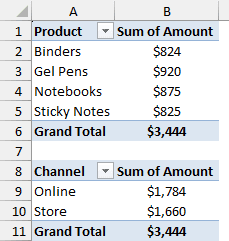
Two PivotTables from the same Sales Table: sales by product and by channel

Now I want one Agent slicer to filter both of them.

First, add a slicer to one PivotTable. Select a cell in the first PivotTable, go to PivotTable Analyze > Insert Slicer, check Agent, and click OK.

My guide to slicers in Excel walks through this in detail.

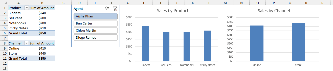
When I click Aisha Khan in the slicer, only the first PivotTable changes. It drops to $850, while the channel PivotTable still shows $3,444.

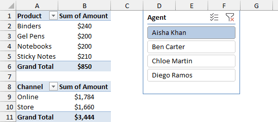
Agent slicer filtering only the first PivotTable

That’s because a new slicer is connected only to the PivotTable you created it from.

Here are the steps to connect the slicer to the second PivotTable:

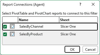
Select the slicer, go to the Slicer tab, and click Report Connections. You can also right-click the slicer and choose Report Connections.
Check the PivotTable you want the slicer to control (SalesByChannel here) and click OK.

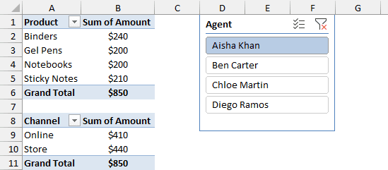
One Agent slicer filtering both PivotTables for Aisha Khan

Now both PivotTables follow the slicer. With Aisha Khan selected, the channel PivotTable shows her $410 of online sales and $440 of store sales.

Note: Report Connections lists only the PivotTables that share a data source with the slicer’s PivotTable. If one is missing, see the troubleshooting section below.

Connecting a Slicer From the PivotTable Side (Filter Connections)

Sometimes it’s easier to start from the PivotTable. This helps when you add a new PivotTable to a report that already has a slicer.

Here are the steps:

Select any cell in the PivotTable you want to connect.
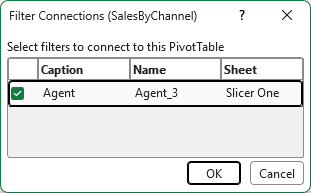
Go to the PivotTable Analyze tab and click Filter Connections. Check the slicer you want to control this PivotTable, then click OK.

Timeline set to Q1 2026 filtering both PivotTables to $2,650

The result is the same as using Report Connections. The dialog just lists slicers instead of PivotTables.

Using One Slicer With Several PivotCharts

A PivotChart always follows its PivotTable. So once a slicer is connected to both PivotTables, it also controls every PivotChart built on them.

Here I’ve added a column chart to each PivotTable. With Aisha Khan selected, both charts show only her sales.

Channel PivotTable built from a range one row short, total $3,220

To add a PivotChart, select a cell in the PivotTable and go to PivotTable Analyze > PivotChart. You don’t need to connect the chart to the slicer separately.

Connecting a Timeline to Multiple PivotTables

A Timeline is a slicer for dates, and it connects to several PivotTables the same way.

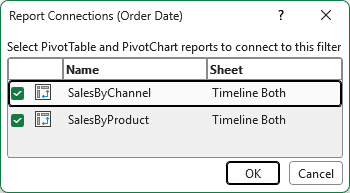
After inserting a Timeline for the Order Date field (PivotTable Analyze > Insert Timeline), right-click it and choose Report Connections. Check the other PivotTable and click OK.

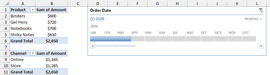
Returns Table with return ID, date, agent, product, qty, and refund

Now pick a date range once, and both PivotTables follow. Here I’ve selected January to March, and both show $2,650 for the first quarter.

Sales and refunds PivotTables built from the Data Model

Connect Slicer to Multiple Pivot Tables (Different Data Sources)

Report Connections can’t help when the PivotTables come from different datasets. For that, you need Excel’s Data Model and a small lookup table that links the datasets.

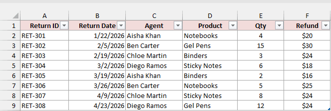
Here I have two Tables. The Sales Table from above, and a Returns Table with eight returned orders.

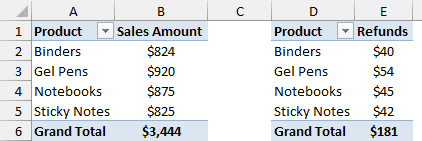
Agent slicer filtering the sales and refunds PivotTables for Aisha Khan

I want one Agent slicer to filter a sales PivotTable and a returns PivotTable together.

The trick is a third table that lists each agent once. Both datasets connect to it, and the slicer comes from it.

Step 1: Build the Agents Lookup Table With Power Query

You could copy the agent names and remove duplicates by hand. But then a new agent never shows up in the slicer until you edit the list.

Power Query builds the list from both Tables and updates it every time you refresh.

Here are the steps:

Go to Data > Get Data > From Other Sources > Blank Query.
In the Power Query Editor, go to Home > Advanced Editor, paste the code below, and click Done.

let
    SalesAgents = Excel.CurrentWorkbook(){[Name="Sales"]}[Content][[Agent]],
    ReturnAgents = Excel.CurrentWorkbook(){[Name="Returns"]}[Content][[Agent]],
    Combined = Table.Combine({SalesAgents, ReturnAgents}),
    Unique = Table.Distinct(Combined),
    Sorted = Table.Sort(Unique, {{"Agent", Order.Ascending}})
in
    Sorted

Rename the query to Agents in the Query Settings pane.

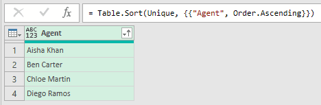
Power Query Editor showing the Agents query with four unique agents

The code takes the Agent column from both Tables, stacks them, and keeps each name once.

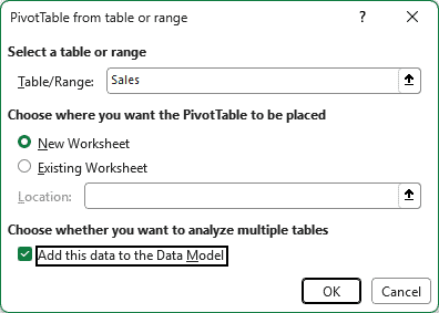
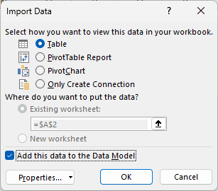
Go to Home, click the Close & Load drop-down, and choose Close & Load To. In the Import Data dialog box, choose Table, check Add this data to the Data Model, and click OK.

Create PivotTable dialog with Add this data to the Data Model checked

Excel loads the four agents to a new sheet as a Table named Agents.

Step 2: Create Both PivotTables in the Data Model

The PivotTables have to come from the Data Model, not straight from the sheet.

Select a cell in the Sales Table and go to Insert > PivotTable.
Check Add this data to the Data Model and click OK.

Report Connections dialog with both PivotTables checked

Build the sales PivotTable as usual (Product in Rows, Amount in Values). Then repeat both steps from the Returns Table to build a refunds PivotTable.

Filter Connections dialog with the Agent slicer checked

Step 3: Create the Relationships

Now tell Excel how the three tables connect. Each dataset links to the Agents table through the Agent column.

Select a cell in either PivotTable and go to PivotTable Analyze > Relationships.
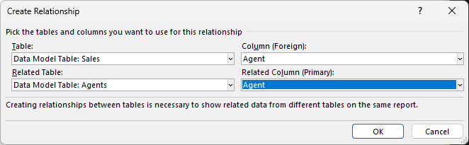
Click New. Pick Data Model Table: Sales as the Table and Agent as the Column (Foreign). Pick Data Model Table: Agents as the Related Table and Agent as the Related Column (Primary). Click OK.

Report Connections dialog for the Order Date timeline

Click New again and create the same relationship for the Returns table. Then click Close.

Note: The Agents table must list each agent only once, and the Agent columns must hold compatible data (text with text, numbers with numbers). Otherwise Excel can’t create the relationship.

Step 4: Insert the Slicer From the Agents Table

The slicer must come from the Agents table, because that’s the one both datasets share.

Select a cell in the sales PivotTable and go to PivotTable Analyze > Insert Slicer.
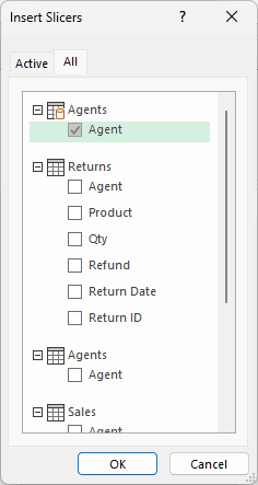
Click the All tab and check Agent under the first Agents entry, then click OK. (Agents is listed twice: the first is the Data Model table, the second is the worksheet Table.)

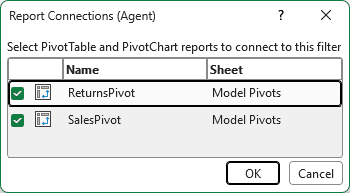
Report Connections dialog listing only one PivotTable

Select the new slicer, go to Slicer > Report Connections, check the returns PivotTable, and click OK.

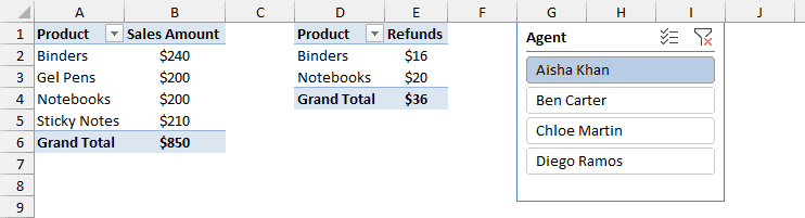
Excel error: disconnect the filter controls before changing the data source

Now click Aisha Khan. The sales PivotTable shows her $850 of sales, and the returns PivotTable shows her $36 of refunds.

Import Data dialog with Table and Add this data to the Data Model

Why a PivotTable Is Missing From Report Connections

If a PivotTable doesn’t show up in the Report Connections list, it isn’t sharing a data source with the slicer’s PivotTable.

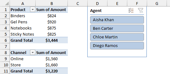
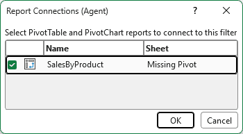
Here’s an example. Both PivotTables look like they use the sales data, but the channel PivotTable reads A1:G16, one row short of the Table.

That’s why its total is $3,220 instead of $3,444.

Create Relationship dialog linking Sales to Agents on Agent

When I open Report Connections for the Agent slicer, only the product PivotTable is listed.

Insert Slicers dialog, All tab, Agent checked under Agents

These are the usual causes:

The PivotTables were built from ranges that differ by even one row or column.
One was built from a Table and the other from a plain range.
One PivotTable is in a different workbook.
One PivotTable uses the Data Model and the other doesn’t. They can never share a slicer.

And these are the fixes:

Build every PivotTable from the same Excel Table. The Table grows with your data, so the source never drifts.
Copy an existing PivotTable and paste it where you need it, then change its fields. The copy shares the original’s source automatically.
For a PivotTable that’s already built, point it to the same Table with PivotTable Analyze > Change Data Source.

Changing the Data Source of a Connected PivotTable

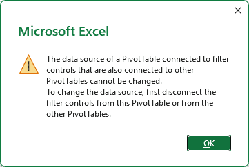
Once a slicer connects two PivotTables, Excel won’t let you change the data source of either one. You get this message:

Report Connections dialog for the Data Model slicer

To change the source, disconnect the slicer first. Open Report Connections, uncheck the PivotTables, change the data source, then connect them again.

Disconnecting a Slicer From a PivotTable

To stop a slicer from filtering a PivotTable, select the slicer, go to Slicer > Report Connections, and uncheck that PivotTable.

You can also do it from the PivotTable side with PivotTable Analyze > Filter Connections.

When you disconnect, Excel removes that slicer’s filter from the PivotTable, so it goes back to showing all the data.

Additional Notes About Connecting Slicers to Multiple Pivot Tables

PivotTables that share a source also share grouping. If you group dates by month in one, the other groups the same way.
The slicer, the PivotTables, and the charts don’t need to be on the same sheet. A slicer on a dashboard sheet can control PivotTables on other sheets.
Refresh after changing the data. In the Data Model setup, Data > Refresh All updates the Agents query, the PivotTables, and the slicer together.
In the example file, the Same Source and Different Sources sheets have everything connected, so you can click the slicers right away.

Frequently Asked Questions

Can two slicers be connected to each other?

Not directly. Connect both slicers to the same PivotTables instead. Then a pick in one slicer fades the items in the other that have no matching data.

Can I connect a slicer to PivotTables in another workbook?

No. A slicer only works with PivotTables in the same workbook. Move the PivotTables into one file first.

Does connecting a slicer to multiple PivotTables work in Excel for the web?

Yes. In Excel for the web, select the slicer and go to Slicer > Slicer Settings. Under PivotTable Connections, check the PivotTables you want it to control.

Does it work on a Mac?

Yes. In Microsoft 365 for Mac, select the slicer, go to the Slicer tab, and click Report Connections, just like on Windows.

Conclusion

I showed you how to connect one slicer to several PivotTables with Report Connections and Filter Connections, and how to add PivotCharts and a Timeline to the same setup.

I also covered PivotTables from different data sources through the Data Model, and what to do when a PivotTable won’t connect. I hope you found this article helpful.

Other Excel articles you may also like:

How to Connect Slicer to Multiple Pivot Tables