Grouping data such as dates, numbers, or text in a Pivot Table can help you to summarize and analyze data more effectively.
Additionally, it can make it easier to identify significant trends and patterns in your data.
However, sometimes when you attempt to group particular data in a Pivot Table, Excel does not display the Grouping dialog box to allow you to group the data but instead shows a warning message indicating that it cannot group that selection.

The “Cannot group that selection” error in Pivot Tables generally indicates a problem with the underlying source data.
This tutorial describes four causes of the ‘Cannot group that selection’ error in Pivot Tables in Excel and offers possible solutions.
Cause #1: Unsupported Date Format
If you have a column of dates, but all or some of the values are in a format not supported by Excel (or are in a text format), you won’t be able to group them by months, quarters, or years.
Also, note that only leap years have a 29th February date; therefore, a 29th February date in a typical year will trigger the “Cannot group that selection” error.
Let’s consider the following Pivot Table with a date in an invalid format in cell A3.

We want to group the dates in column A by months using the steps below:
- Select any date in column A, right-click the selection, and choose Group on the shortcut menu.
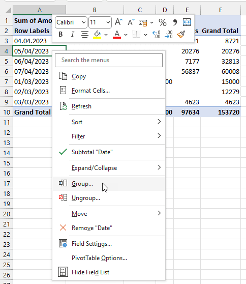
Excel does not display the Grouping dialog box to allow you to group the dates but instead shows a warning message indicating it cannot group that selection (as shown below).

How to Fix this ‘Cannot Group that selection‘ error
The only way to fix this error is to reenter the invalid date in the source dataset in a format supported by Excel. You can then refresh the Pivot Table and then group the data again.
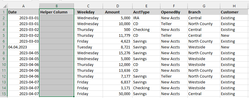
However, it can be challenging in a large dataset to spot the cell or cells with invalid dates easily. You can use the below steps to make it easy to identify the cells with dates in a format unsupported by Excel:
- Insert a helper column in the source dataset as shown in the example dataset below:
- Select cell B2 and enter the formula =A2+1. This formula adds the value 1 to the data in cell A2.
- Double-click or drag the fill handle feature to copy the formula down the column.

The formula returns the #VALUE! Error if the referenced cell contains a date in a format unsupported by Excel.
In this case, the date in cell A7 has an invalid format, and we need to fix it. Therefore, we reenter the date in the format “yyyy-mm-dd,” as shown below:

Notice that cell B7 no longer has the #VALUE! error. We can now delete the helper column.
- Right-click any cell on the Pivot Table, and click Refresh on the shortcut menu. This will refresh the Pivot Table and show us the changes that we made in the source data

- Right-click any cell with a date on column A and choose Group on the shortcut menu.

Because all the dates are in a format supported by Excel, Excel now returns the Grouping dialog box.
- Select Months on the Grouping dialog box and click OK.

Note: You can change the starting and ending dates on the Grouping dialog box if the default values are unsuitable for your work.
The dates on column A of the Pivot Table are now grouped by months:

How to Filter the Cells With #VALUE! Error
We have only one #VALUE! error in the helper column. However, sometimes you can have many cells with the value error.

If there are many cells with the value error, you can filter the cells to quickly review and fix the errors without unnecessarily scrolling the worksheet.
You can use the steps below to filter the cells with the value error:
- Select the cell range B1:B15 in the helper column.
- On the Data tab, click the Filter button on the Sort & Filter group.

- Open the filter drop-down in cell B1, and deselect all the options in the bottom area except the #VALUE! option and click OK.

The cells with the value error are selected, and you can now quickly review the errors and fix them accordingly.

Also read: How to Fix Pivot Table Field Name is Not Valid Issue
Cause #2: Text Strings in a Numeric Column
If you have a column that is supposed to contain only numeric values, but some are text strings, you won’t be able to group the values in a Pivot Table.
Suppose we have the following Pivot Table with a text string that looks like a number in cell A15.

We want to group the values in column A in groups of 10,000s. We use the steps below:
- Right-click any number in column A of the Pivot Table and choose Group on the shortcut menu.

Excel does not group the data and displays the warning message that it cannot group that selection.

How to Fix this ‘Cannot Group that selection‘ error
To fix the error, ensure that all the entries in the underlying column are numbers. Next, refresh the Pivot Table and then group the data.
However, spotting the cell or cells with text strings can be challenging in a large dataset. You can use the below steps to make it easy to identify the cells with text strings, especially those that look like numbers:
- Insert a helper column in the source dataset.

- Select cell D2 and enter the following formula:
=ISNUMBER(C2)
Note: The ISNUMBER function checks whether a given value is a number. The function returns TRUE if the value is a number and FALSE if not.

- Drag or double-click the fill handle feature to copy the formula down the column.

The formula returns FALSE in cell D3 because the value in cell C3 is not a number but a text string.
Notice that the value in cell C3 has a space between the digit 1 and the zeroes. So it looks like the number 1000, but it is a test string.
Remove the space between the digit 1 and the zeroes, and the value becomes a number.

We can now turn to the Pivot Table and do the following steps:
- Right-click any cell on the Pivot Table and click Refresh on the shortcut menu.

- Right-click any cell with a number in column A of the Pivot Table and choose Group on the shortcut menu.

- Click OK on the Grouping dialog box to accept the default settings.

Note: You can change the default settings if they are unsuitable for your work.
The numbers in column A of the Pivot Table are now grouped.

Note: In case you have blank cells in the columns, it would also be treated as text and you would see the error prompt
Also read: Delete a Pivot Table in Excel
Cause #3: The Column You Want to Group is a Text Column
While you can group text items in a column in Pivot Table, you need to select the items you want to group and then click on the group option.
Unlike the grouping of a column with numbers, if you just right-click on one cell and then use the group option, it will show you the prompt that says that it can not group these items (which is because it does not know what items to group together).
Suppose we have the following Pivot Table with a text column A.

We want to group the first three items in column A into “New Branches” and the last two into “Old Branches.”
If I right-click on any single cell and then click on the Group option (as shown below), it will show the error prompt:

How to Fix this ‘Cannot Group that selection‘ error
You need to manually select the text items in column A of the Pivot Table that you want to group and then group them.
To do that, use the steps below:
- Select the first three branches in cells A5, A6, and A7. Right-click the selection and choose Group on the shortcut menu.

A default Group1 is automatically created:

Not that any cell that is not in the selected group would automatically be assigned to a default group of its own. For example, South is automatically assigned to a group called South.
- Select cell A10, press and hold down the Ctrl key and select cell A12. Right-click the selection and choose Group on the shortcut menu.

A default Group2 is automatically created:

- Rename the groups by selecting cells A5 and A9 and typing “New Branches” and “Old Branches,” respectively.

Also read: Lock Pivot Table Column Width
Cause #4: Pivot Table Was Added to a Data Model
If you select the Add this data to the Data Model check box when creating a Pivot Table,

…you won’t be able to group items on the Pivot Table:

How to Fix this ‘Cannot Group that selection‘ error
Create another Pivot Table based on the same source data but do not select the Add this data to the Data Model check box.
This tutorial explained four causes of the “Cannot group that selection” error in Pivot Tables and offered possible solutions. We hope you found the tutorial helpful.
Other Excel articles you may also like: