A Pivot Table is an interactive table that can summarize vast amounts of numeric data enabling us to analyze data in finer detail.
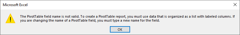
Therefore it can be frustrating when you try to create or refresh a Pivot Table, and Excel returns a warning message box with the message,
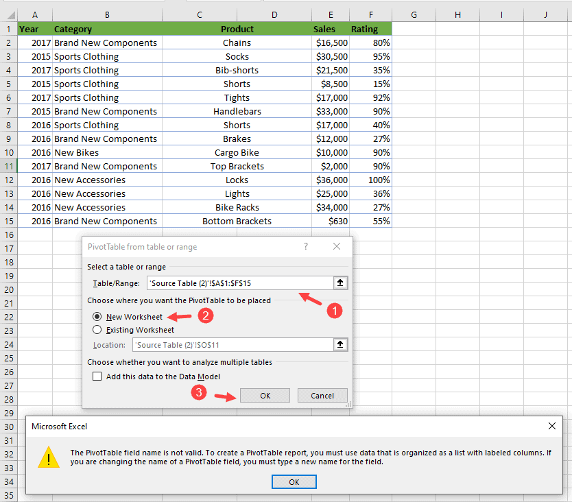
“The PivotTable field name is not valid. To create a PivotTable report, you must use data that is organized as a list with labeled columns. If you are changing the name of a PivotTable field, you must type a new name for the field.”
As much as Excel offers some information to help fix the problem, we may need clarification about what to do to resolve the issue.
In this tutorial, I will show you five ways of fixing the “Pivot Table field name is not valid” error.
Method #1: Ensure that Every Column in The Source Data Range is Labeled
Excel does not allow inserting a Pivot Table if the source data range has a column or columns without column labels.
Therefore, we must ensure that all the data range columns have labels before inserting a Pivot Table.
Let’s attempt to create a Pivot Table based on the following data range that does not have a column label in cell C1.

Below are the steps to create a Pivot Table using the above dataset:
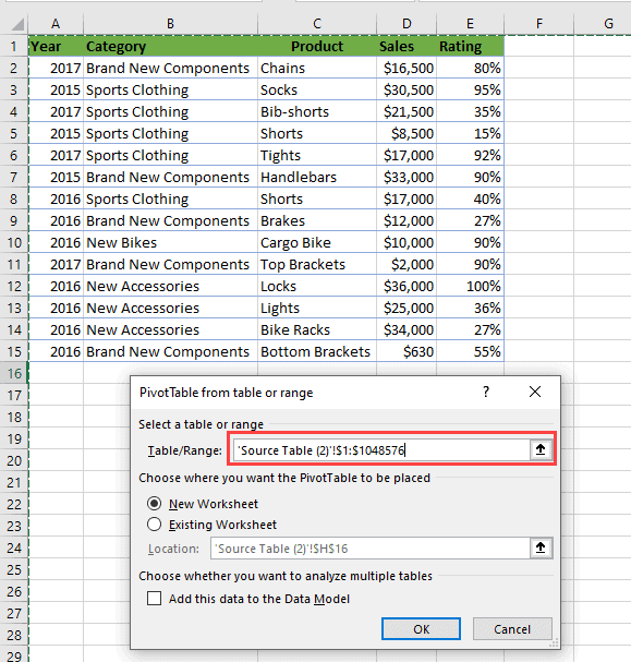
- Click the Insert tab and select From Table/Range option on the Pivot Table drop-down.

- In the dialog box that appears, click the Range Selector button in the Table/Range box.
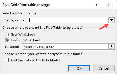
- Select range A1:E15.

- Click the Range Selector button again to expand the dialog box. Select the New Worksheet option and click OK.

Excel immediately returns the following warning message box:

Click OK on the message box and click Cancel on the Pivot Table from table or range dialog box to dismiss it.
To fix this issue, we need to insert a column label in cell C1.

We can now create the following Pivot Table from the data range A1:E15:
Note: A column label in the source data range may be mistakenly deleted after successfully inserting a Pivot Table. If you try to refresh the Pivot Table by clicking the Refresh button on the Pivot Table Analyze tab,

You get the error message:

To fix the problem, go back to the source range and type in the deleted column label. You will then be able to refresh the Pivot Table successfully.
Also read: Cannot Group That Selection Error in Excel Pivot Tables
Method #2: Unmerge Cells in the Source Data Range
Sometimes we merge cells in our dataset; that is, we join one or more cells into one big cell.
We do this when for example, we want to create labels that span several columns.
If you try to create a Pivot Table based on a data range that has merged cells, Excel returns the ‘Pivot Table field name is not valid‘ warning message.
The following dataset has merged cells in columns C and D.

If you try to create a Pivot Table based on this data range, Excel returns the warning message that the Pivot Table field name is not valid.
To fix this problem, select range C2:D15, click the Home tab, and select the Unmerge Cells option in the Alignment group.

The cells are unmerged, resulting in an empty column D.

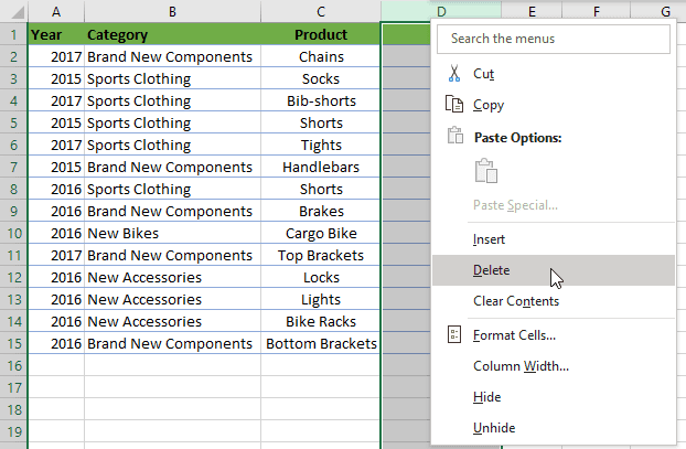
Right-click the letter header of column D and select Delete on the shortcut menu that appears:
We should now be able to create a Pivot Table based on the data range that does not have merged cells.
Also read: Merge or Unmerge Cells in Excel (Shortcut)
Method #3: Restore the Deleted Source Table/Date Range
One may inadvertently delete the data range after inserting a Pivot Table.
If you try to refresh a Pivot Table based on a deleted Table or Data range, you will get the warning message that the Pivot table field name is not valid.
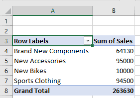
For example, we have the following Pivot Table:

Let’s delete its source data range:

Right-click any cell in the Pivot Table and select Refresh on the shortcut menu that appears:

Instead of the Pivot Table getting refreshed, we get the warning message that the Pivot Table field name is not valid.

We can solve this problem by restoring the source data range to its original location.
In this case, open the worksheet that contained the deleted data range and press Ctrl + Z to restore the data range.
We can then refresh the Pivot Table successfully.
Also read: Change Count to Sum in Excel Pivot Table
Method #4: Select Only the Data Range with Data, Not the Entire Worksheet
Sometimes those who are just beginning to create Pivot Tables in Excel make the mistake of selecting the entire worksheet instead of only the data range with data.
This usually happens when they press the Select All button in the top left corner of the worksheet when selecting the source range:

This results in the warning message that the Pivot Table field name is not valid.
Only select the source range with data to avoid the field name is not valid error while creating the Pivot Table.
Also read: Data Source Reference is Not Valid Error in Excel
Method #5: Delete Empty Columns in Source Data Range
Sometimes after inserting a Pivot Table, one may mistakenly insert empty columns in the source data range.
Then, when you try to refresh the Pivot Table, you get the warning message that the Pivot field name is not valid.
For example, we have the following Pivot Table.

Let’s insert an empty column in its source data range:

Right-click any cell in the Pivot Table and select Refresh on the shortcut menu that appears:

Instead of the Pivot Table getting refreshed, we get the warning message that the Pivot Table field name is not valid.

We need to delete the empty column so that the Pivot Table can be refreshed.
Right-click the letter header of the blank column and select Delete on the shortcut menu that appears.

We can then refresh the Pivot Table successfully.
This tutorial has shown various ways of resolving the “Pivot Table field name is not valid” error in Excel. The methods include:
- Label any column in the source data range that does not have a label.
- Unmerge all merged cells in the data range.
- Restore the deleted data range.
- Delete any blank columns in the data range.
I hope this tutorial helped you in getting an understanding of why you were getting the error and how to fix it.
Other Excel articles you may also like: