Conditional Formatting in Excel provides a great way to highlight certain cells that may be more important than others.
When combined with the OR criterion, you get added flexibility to your formatting condition options.
In this tutorial, we will see how to use conditional formatting, specifically with the OR criteria.
What is Conditional Formatting in Excel?
Conditional formatting allows you to apply particular formatting to only those cells that satisfy the given criteria.
Most often it is to apply color-based formatting to highlight, emphasize, or differentiate among data and information stored in a spreadsheet.
The great thing about conditional formatting is that it lets you specify the condition or criteria for formatting in a multitude of ways. You can use it to format:
- Cells that contain duplicate or unique values
- Cells that contain a particular value
- Cells that contain a particular range of values
- Cells that return true for a particular formula
…and more.
In this tutorial, we will be applying conditional formatting using a formula. This means that Excel will decide which cells to format based on the result of a formula.
Also read: Copy Conditional Formatting in Excel
What are Logical Functions in Excel?
Logical functions like OR, AND and NOT let you carry out more than one comparison, or test multiple conditions. The function returns a logical value based on the set of conditions, which can be either TRUE or FALSE.
The OR function returns a TRUE if any of the conditions operated on is TRUE. So, you can have an OR function with the following syntax:
=OR(condition1,condition2,[condition3],..)
where condition1, condition2, etc. are conditions with comparison operators like =, <, <=, >, or <=. The OR function will return TRUE even if one of the conditions is true.
Example to Explain How to Use Conditional Formatting with OR Criteria
Now let us see how to combine the two concepts discussed – Conditional Formatting with OR Criteria. To explain this, we will use a sample problem.
Using Conditional Formatting with OR Criteria
When you include an OR function in a conditional formatting rule, you can highlight cells in the table that satisfy at least one of the conditions defined in the OR function.
Let us say you have a set of Employee Names, Departments, and Sales values as shown in the screenshot below:
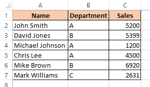
If you want to highlight all the rows where an employee is from department B or has Sales of more than $5000, you can use Conditional Formatting with OR criteria as follows:
- Select all the cells where you want to apply cell formatting. In our case, we select the range A2:C7.
- Under the Home tab, click on the Conditional Formatting button (in the Styles group).

- This will display a drop-down menu with different conditional formatting options. Select ‘New Rule’.

- This will open the ‘New Formatting Rule’ dialog box.
- From the options under ‘Select a Rule Type’, click on the option ‘Use a formula to determine which cells to format’.

- This will open a new section below to edit the rule description. In the input box below ‘Format values where this formula is true’, type the formula: =OR($B2=”B”,$C2>5000)

- Next, you need to specify what formatting you want to apply to the row if its values return TRUE for the above formula. Click on the Format button.

- This will open the ‘Format Cells’ dialog box from where you can apply whatever formatting you want to apply to the selected rows.
- We just want to highlight the rows with a yellow fill color, so we can select the ‘Fill’ tab and select the Yellow color from the Background color options shown.

- Click OK to close the Format Cells dialog box.

- Click OK again to close the New Formatting Rule dialog box.

- All the rows that satisfy the condition (have either the department as B or Sales more than $5000) will be highlighted with a yellow background color.

You can apply this method with as many conditions and as many types of conditions as you need to. You can also follow the same technique with other comparison functions like AND and NOT.
In this tutorial, I showed you step by step how to use conditional formatting with OR criteria to highlight data in a table if at least one of the given conditions is met.
I hope you can use the method explained in this tutorial for your own data and applications, to get your required formatting results.
Other Excel tutorials you may also like:
- How to Find Duplicates in Excel (Conditional Formatting/ Count If/ Filter)
- How to Highlight Every Other Row in Excel (Conditional Formatting & VBA)
- Highlight Cell If Value Exists in Another Column in Excel
- How to Hide Rows based on Cell Value in Excel
- How to Copy Formatting In Excel
- How to Highlight Duplicates in Excel