Working with large datasets that contain rows after rows of data can be quite painful.
In such cases, looking for data that match particular criteria can be like looking for a needle in a haystack.
Thankfully, Excel provides some features that let you hide certain rows based on the cell value so that you only see the rows that you want to see. There are two ways to do this:
- Using filters
- Using VBA
In this tutorial, we will discuss both methods, and you can pick the method you feel most comfortable with.
Using Filters to Hide Rows based on Cell Value
Let us say you have the dataset shown below, and you want to see data about only those employees who are still in service.

This is really easy to do using filters. Here are the steps you need to follow:
- Select the working area of your dataset.
- From the Data tab, select the Filter button. You will find it in the ‘Sort and Filter’ group.

- You should now see a small arrow button on every cell of the header row.
- These buttons are meant to help you filter your cells. You can click on any arrow to choose a filter for the corresponding column.
- In this example, we want to filter out the rows that contain the Employment status = “In service”. So, select the arrow next to the Employment Status header.
- Uncheck the boxes next to all the statuses, except “In service”. You can simply uncheck “Select All” to quickly uncheck everything and then just select “In service”.

- Click OK.
You should now be able to see only the rows with Employment Status=”In service”. All other rows should now be hidden.

Note: To unhide the hidden cells, simply click on the Filter button again.
Also read: Change Cell Color Based on Value of Another Cell in Excel
Using VBA to Hide Rows based on Cell Value
The second method requires a little coding. If you are accustomed to using macros and a little coding using VBA, then you get much more scope and flexibility to manipulate your data to behave exactly the way you want.
Writing the VBA Code
The following code will help you display only the rows that contain information about employees who are ‘In service’ and will hide all other rows:
Sub HideRows()
StartRow = 2
EndRow = 19
ColNum = 3
For i = StartRow To EndRow
If Cells(i, ColNum).Value <> "In service" Then
Cells(i, ColNum).EntireRow.Hidden = True
Else
Cells(i, ColNum).EntireRow.Hidden = False
End If
Next i
End SubThe macro loops through each cell of column C and hide the rows that do not contain the value “In service”. It should essentially analyze each cell from rows 2 to 19 and adjust the ‘Hidden’ attribute of the row that you want to hide.
To enter the above code, copy it and paste it into your developer window. Here’s how:
- From the Developer menu ribbon, select Visual Basic.

- Once your VBA window opens, you will see all your files and folders in the Project Explorer on the left side. If you don’t see Project Explorer, click on View->Project Explorer.

- Make sure ‘ThisWorkbook’ is selected under the VBA project with the same name as your Excel workbook.

- Click Insert->Module. You should see a new module window open up.

- Now you can start coding. Copy the above lines of code and paste them into the new module window.

- In our example, we want to hide the rows that do not contain the value ‘In service’ in column 3. But you can replace the value of ColNum number from “3” in line 4 to the column number containing your criteria values.
- Close the VBA window.
Note: If your dataset covers more than 19 rows, you can change the values of the StartRow and EndRow variables to your required row numbers.
If you can’t see the Developer ribbon, from the File menu, go to Options. Select Customize Ribbon and check the Developer option from Main Tabs.
Finally, Click OK.
Your macro is now ready to use.
Running the Macro
Whenever you need to use the above macro, all you need to do is run it, and here’s how:
- Select the Developer tab
- Click on the Macros button (under the Code group).

- This will open the Macro Window, where you will find the names of all the macros that you have created so far.
- Select the macro (or module) named ‘HideRows’ and click on the Run button.

You should see all the rows where Employment Status is not ’In service’ hidden.

Explanation of the Code
Here’s a line by line explanation of the above code:
- In line 1 we defined the function name.
Sub HideRows()
- In lines 2, 3 and 4 we defined variables to hold the starting row and ending row of the dataset as well as the index of the criteria column.
StartRow = 2
EndRow = 19
ColNum = 3
- In lines 5 to 11, we looped through each cell in column “3” (or column C) of the Active Worksheet. If a cell does not contain the value “Inservice”, then we set the ‘Hidden’ attribute of the entire row (corresponding to that cell) to True, which means we want to hide the entire corresponding row.
For i = StartRow To EndRow
If Cells(i, ColNum).Value <> "In service" Then
Cells(i, ColNum).EntireRow.Hidden = True
Else
Cells(i, ColNum).EntireRow.Hidden = False
End If
Next i- Line 12 simply demarcates the end of the HideRows function.
End Sub
In this way, the above code hides all the rows that do not contain the value ‘In service’ in column C.
Also read: Check If Value is in List in Excel
Un-hiding Rows Based On Cell Value
Now that we have been able to successfully hide unwanted rows, what if we want to see the hidden rows again?
Doing this is quite easy. You only need to make a small change to the HideRows function.
Sub UnhideRows()
StartRow = 2
EndRow = 19
ColNum = 3
For i = StartRow To EndRow
Cells(i, ColNum).EntireRow.Hidden = False
Next i
End SubHere, we simply ensured that irrespective of the value, all the rows are displayed (by setting the Hidden property of all rows to False).
You can run this macro in exactly the same way as HideRows.

Hiding Rows Based On Cell Values in Real-Time
In the first example, the columns are hidden only when the macro runs. However, most of the time, we want to hide columns on-the-fly, based on the value in a particular cell.
So, let’s now take a look at another example that demonstrates this. In this example, we have the following dataset:
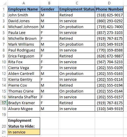
The only difference from the first dataset is that we have a value in cell A21 that will determine which rows should be hidden. So when cell A21 contains the value ‘Retired’ then only the rows containing the Employment Status ‘Retired’ are hidden.
Similarly, when cell A21 contains the value ‘On probation’ then only the rows containing the Employment Status ‘On probation’ are hidden.
When there is nothing in cell A21, we want all rows to be displayed.
We want this to happen in real-time, every time the value in cell A21 changes. For this, we need to make use of Excel’s Worksheet_SelectionChange function.
The Worksheet_SelectionChange Event
The Worksheet_SelectionChange procedure is an Excel built-in VBA event
It comes pre-installed with the worksheet and is called whenever a user selects a cell and then changes his/her selection to some other cell.
Since this function comes pre-installed with the worksheet, you need to place it in the code module of the correct sheet so that you can use it.
In our code, we are going to put all our lines inside this function, so that they get executed whenever the user changes the value in A21 and then selects some other cell.
Writing the VBA Code
Here’s the code that we are going to use:
StartRow = 2
EndRow = 19
ColNum = 3
For i = StartRow To EndRow
If Cells(i, ColNum).Value = Range("A21").Value Then
Cells(i, ColNum).EntireRow.Hidden = True
Else
Cells(i, ColNum).EntireRow.Hidden = False
End If
Next iTo enter the above code, you need to copy it and paste it in your developer window, inside your worksheet’s Worksheet_SelectionChange procedure. Here’s how:
- From the Developer menu ribbon, select Visual Basic.
- Once your VBA window opens, you will see all your project files and folders in the Project Explorer on the left side.
- In the Project Explorer, double click on the name of your worksheet, under the VBA project with the same name as your Excel workbook. In our example, we are working with Sheet1.

- This will open up a new module window for your selected sheet.
- Click on the dropdown arrow on the left of the window. You should see an option that says ‘Worksheet’.

- Click on the ‘Worksheet’ option. By default, you will see the Worksheet_SelectionChange procedure created for you in the module window.

- Now you can start coding. Copy the above lines of code and paste them into the Worksheet_SelectionChange procedure, right after the line: Private Sub Worksheet_SelectionChange(ByVal Target As Range).

- Close the VBA window.
Running the Macro
The Worksheet_SelectionChange procedure starts running as soon as you are done coding. So you don’t need to explicitly run the macro for it to start working.
Try typing the ‘Retired’ in the cell A21, then clicking any other cell. You should find all rows containing the value ‘Retired’ in column C disappear.

Now try replacing the value in cell A21 to ‘On probation’, then clicking any other cell. You should find all rows containing the value ‘On probation’ in column C disappear.

Now try removing the value in cell A21 and leaving it empty. Then click on any other cell. You should find both rows become visible again.

This means the code is working in real-time when changes are made to cell B20.
Explanation of the Code
Let us take a few minutes to understand this code now.
- Lines 1, 2, and 3 define variables to hold the starting row and ending row of the dataset as well as the index of the criteria column. You can change the values according to your requirement.
StartRow = 2
EndRow = 19
ColNum = 3
- Lines 4 to 10, loop through each cell in column “3” (or column C) of the worksheet. If the cell contains the value in cell A21, then we set the ‘Hidden’ attribute of the entire row (corresponding to that cell) to True, which means we want to hide the entire corresponding row.
For i = StartRow To EndRow
If Cells(i, ColNum).Value = Range("A21").Value Then
Cells(i, ColNum).EntireRow.Hidden = True
Else
Cells(i, ColNum).EntireRow.Hidden = False
End If
Next iIn this way, the above code hides the rows of the dataset depending on the value in cell A21. If A21 does not contain any value then the code displays all rows.
In this tutorial, I showed you how you can use Filters as well as Excel VBA to hide rows based on a cell value.
I did this with the help of two simple examples – one that removes required rows only when the macro is explicitly run and another that works in real-time.
I hope that we have been successful in helping you understand the concept behind the code so that you can customize it and use it in your own applications.
Other Excel tutorials you may also like:
- How to Hide Columns Based On Cell Value in Excel
- How to Delete Filtered Rows in Excel (with and without VBA)
- How to Highlight Every Other Row in Excel (Conditional Formatting & VBA)
- How to Unhide All Rows in Excel with VBA
- How to Set a Row to Print on Every Page in Excel
- How to Paste in a Filtered Column Skipping the Hidden Cells
- How to Select Multiple Rows in Excel
- How to Select Rows with Specific Text in Excel
- How to Move Row to Another Sheet Based On Cell Value in Excel?
- How to Compare Two Cells in Excel?
Great advice – works perfectly.
Glad you found the article helpful!