
If you enter data in Excel often, a drop-down list can save time.
With the drop-down, you pick an option instead of typing it. That helps prevent typos and wrong entries.
In this article, I’ll show you how to create basic drop-down lists, lists that update as you add items, and dependent drop-downs.
Create a Basic Drop-Down List in Excel
The easiest way to create a drop-down is through Excel’s Data Validation dialog box. From there, you can tell Excel where to find the choices.
- Type a short set of choices directly into the dialog box.
- Keep the choices in cells on the same sheet or a separate sheet.
- Give the cells holding the choices a name, then use that name for the drop-down.
Method #1: Typing the Items in Data Validation
For a short list that rarely changes, I would start by typing the choices directly into Data Validation.
Below I have travel requests on the Typed List sheet. A1:C11 contains the Request ID, Employee, and Travel Mode columns.
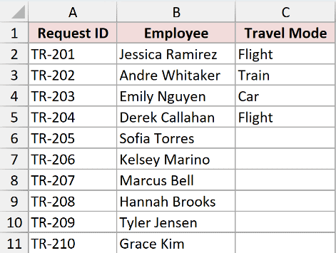
The requests run from TR-201 to TR-210. In C2:C5, I have Flight, Train, Car, and Flight. C6:C11 is blank.
I want you to be able to choose Flight, Train, Car, or Bus in every request cell from C2:C11.
Here’s how to create the list:
- Select C2:C11, then go to the Data tab > Data Validation.
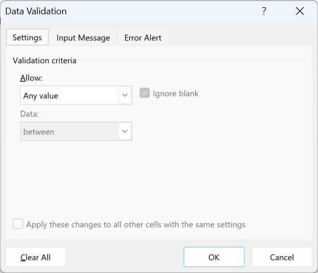
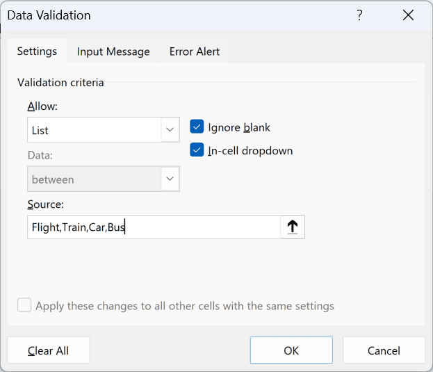
- On the Settings tab, choose List under Allow. In Source, type
Flight,Train,Car,Bus. Keep In-cell dropdown checked, then click OK.
Now when you click a cell in C2:C11 and open its arrow, you can choose any of the four travel modes, including Bus.
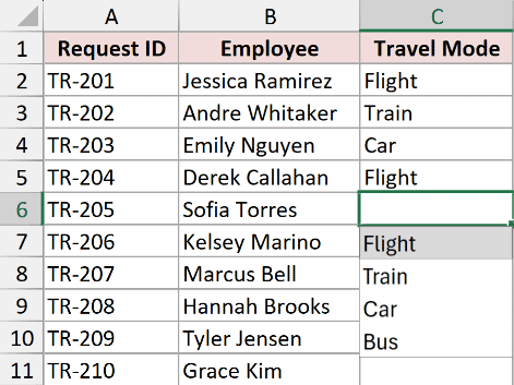
Your existing entries stay in place. Excel doesn’t fill the blank cells when you add the drop-down, so you still need to choose each travel mode.
Note: To change the choices later, reopen Data Validation and edit the Source box. This works for a few fixed choices, but a long typed list gets tedious to maintain.
Method #2: Using a Cell Range
If you’d rather keep the choices on the worksheet, type them in cells and use those cells for the drop-down. You can edit the list without reopening Data Validation.
Below I have travel requests in A1:C11 on the Cell Range sheet. I keep the Departments list in E1:E7.
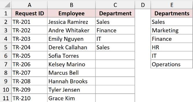
In E2:E7, I have Sales, Marketing, Finance, HR, IT, and Operations. C2:C5 already contains Sales, Finance, IT, and Sales.
Here’s how to add the department drop-down:
- Select C2:C11 and go to the Data tab > Data Validation. On the Settings tab, choose List under Allow.
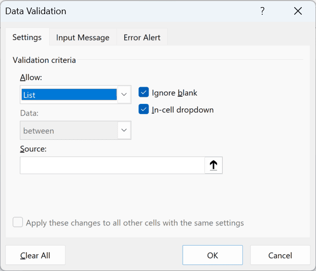
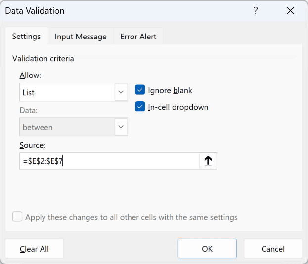
- Click inside Source, then select E2:E7. Check that Source reads
=$E$2:$E$7, keep In-cell dropdown checked, and click OK.
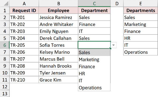
Now when you click any cell in C2:C11, you’ll see all six departments from E2:E7.
The dollar signs keep the source fixed on those cells. Excel adds them for you when you select the range in the dialog.
If you change a department within E2:E7, the available choice changes too. For new departments below the range, extend the source or use the Excel Table method.
Method #3: Using a List on Another Sheet
If you want more room for the request data, keep the choices on a separate sheet.
Below I have travel requests on the Other Sheet sheet. A1:C11 contains the Request ID, Employee, and Destination columns.
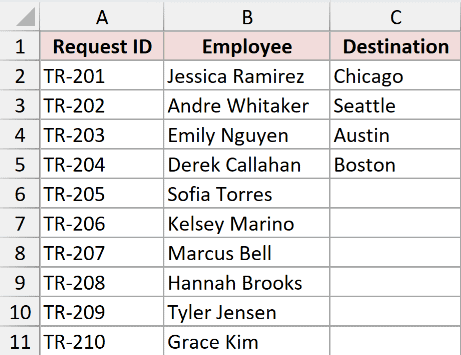
In C2:C5, I have Chicago, Seattle, Austin, and Boston. I keep the source cities on the Lists sheet under the Cities heading in A1.
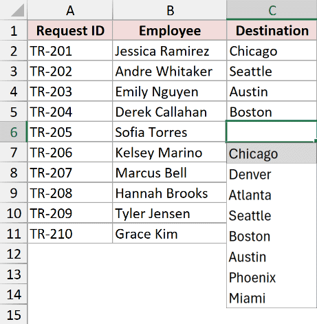
On Lists, A2:A9 contains Chicago, Denver, Atlanta, Seattle, Boston, Austin, Phoenix, and Miami.
Here’s how to use the list from the other sheet:
- On Other Sheet, select C2:C11. Open Data tab > Data Validation, then choose List under Allow on the Settings tab.
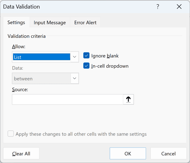
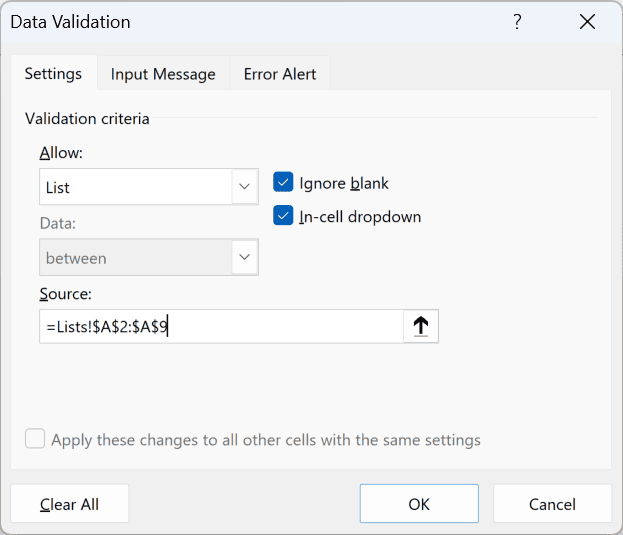
- Click inside Source, click the Lists sheet tab, and select A2:A9. The Source should read
=Lists!$A$2:$A$9. Click OK.
Now when you open the Destination drop-down on Other Sheet, you’ll see the eight cities from Lists.
I find this arrangement useful when several entry sheets share the same choices. You only have one city list to maintain.
Note: You can hide the Lists sheet after you set up the drop-down. The list will keep working, and you can unhide the sheet when you need to edit it.
Method #4: Using a Named Range
If you want the same choices in several drop-downs, give the cells holding them a name. That name is easier to recognize than a cell address.
Below I have travel requests in A1:C11 on the Named Range sheet. I keep the Approvers list in E1:E5.
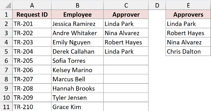
In E2:E5, I have Linda Park, Robert Hayes, Nina Alvarez, and Chris Dalton. C2:C5 contains Linda Park, Nina Alvarez, Robert Hayes, and Linda Park.
Here’s how to name the source and use it:
- Select E2:E5. Click the Name Box to the left of the formula bar, type Approvers, and press Enter.
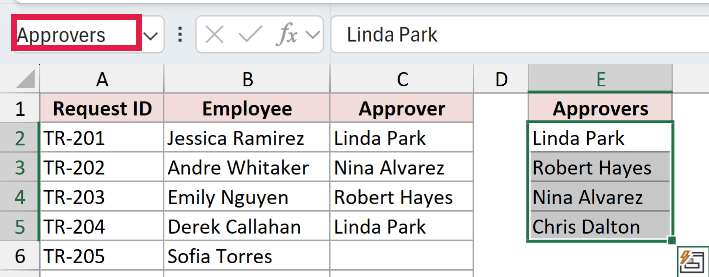
Excel creates Approvers for the whole workbook. It points to ='Named Range'!$E$2:$E$5 and works on any sheet. You can create it through Formulas > Define Name.
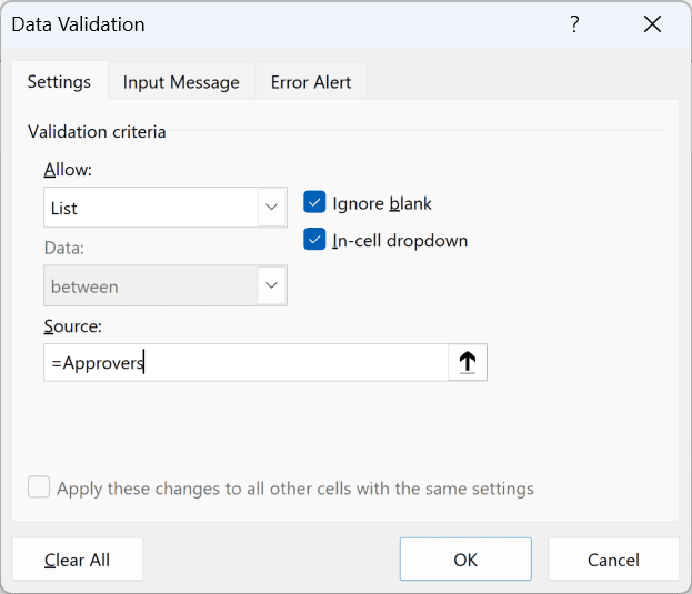
- Select C2:C11 and open Data tab > Data Validation. Choose List under Allow, enter
=Approversin Source, and click OK.
Now when you open an Approver cell, you’ll see Linda Park, Robert Hayes, Nina Alvarez, and Chris Dalton.
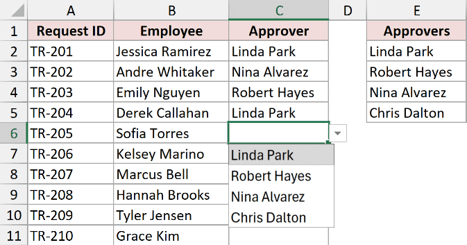
The name makes the drop-down source easier to read, but it doesn’t make the list grow. It still points only to E2:E5.
Note: Range names can’t contain spaces. Create the name for the whole workbook when the same source needs to work on different sheets.
Create a Drop-Down List That Updates Automatically
If you add choices later, the drop-down can grow with them. I’ll show you how to update the choices with an Excel Table or a formula.
Method #5: Using an Excel Table
If you add departments often, turn the department list into an Excel Table. The table grows as you add items, so you don’t have to edit Data Validation each time.
This is the method I recommend for most people. It works in Excel 2007 onwards and needs no formulas.
Below I have travel requests in A1:C11 on the Excel Table sheet. I keep the Departments list in E1:E7.
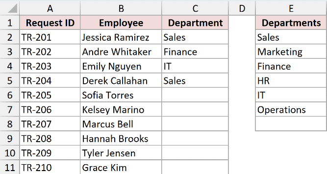
In E2:E7, I have Sales, Marketing, Finance, HR, IT, and Operations. C2:C5 already contains Sales, Finance, IT, and Sales.
Here’s how to make the drop-down grow with its source:
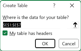
- Select E1:E7 and press Ctrl+T. Check My table has headers and click OK. On the Table Design tab, change Table Name to DeptList.
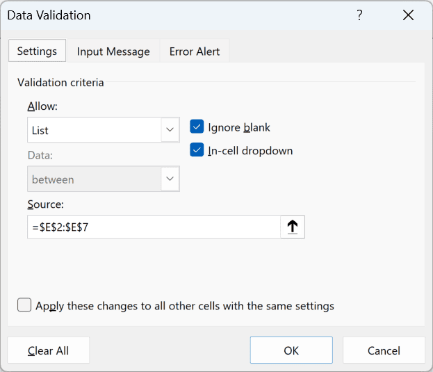
- Select C2:C11 and open Data tab > Data Validation. Choose List under Allow, then select the table’s data cells E2:E7 for Source. Confirm
=$E$2:$E$7and click OK.
- Type Legal in E8, directly underneath the table, and press Enter.
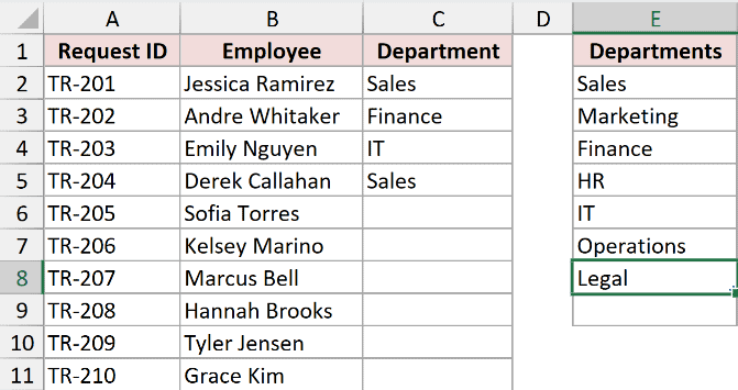
When the table expands to E8, the validation Source becomes =$E$2:$E$8. Now you’ll see seven departments in the drop-down, including Legal.
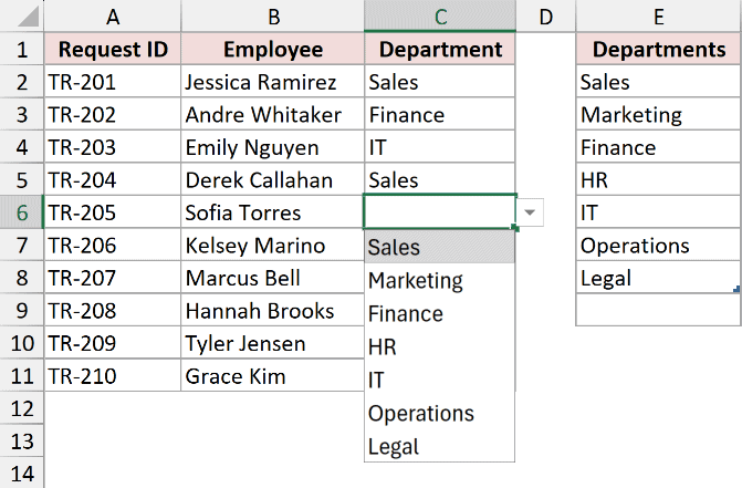
From here, you only need to maintain the department list. The request cells will keep using the expanded source.
Note: Add each new item directly beneath the table with no blank row. Before you check the drop-down, confirm that the table expanded to include it.
Method #6: Using UNIQUE and a Spill Reference (Microsoft 365)
If your source log contains repeated entries, here’s a cleaner option. A formula can build a sorted list without duplicates.
You can use this method in Microsoft 365 and Excel 2021 or later.
Below I have a travel log in A1:C11 on the Unique List sheet, with repeated destinations in column C.
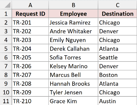
In C2:C11, I have Chicago, Denver, Chicago, Atlanta, Seattle, Denver, Boston, Atlanta, Chicago, and Austin.
On the New Request card, G1 contains New Request, H1 contains Destination, and G2 contains TR-211. I want H2 to offer each logged city once.
Here’s how to build the choices and connect them to the card:
- Enter Unique Cities in E1. In E2, enter the following formula and press Enter.
=SORT(UNIQUE(C2:C11))
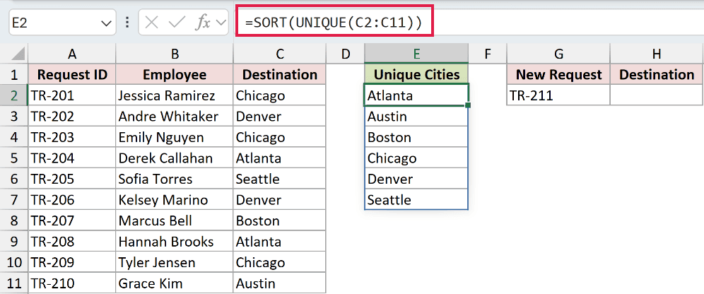
How does this formula work?
UNIQUE removes the repeated cities from C2:C11. Then SORT puts the remaining cities in alphabetical order.
Excel fills E2:E7 with Atlanta, Austin, Boston, Chicago, Denver, and Seattle. You don’t need to copy the formula down.
- Select H2 and open Data tab > Data Validation. Choose List under Allow, enter
=$E$2#in Source, and click OK.
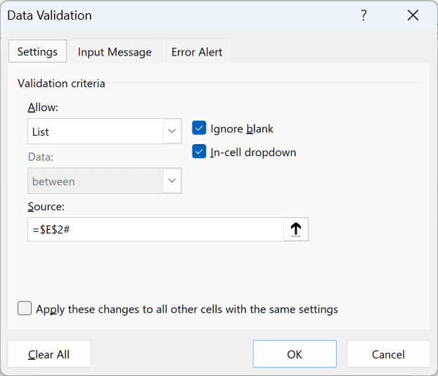
The # tells Excel to use every result produced from E2. If the formula returns more or fewer cities, the drop-down follows those results.
Now when you open H2 for request TR-211, you’ll see the six unique cities in alphabetical order.
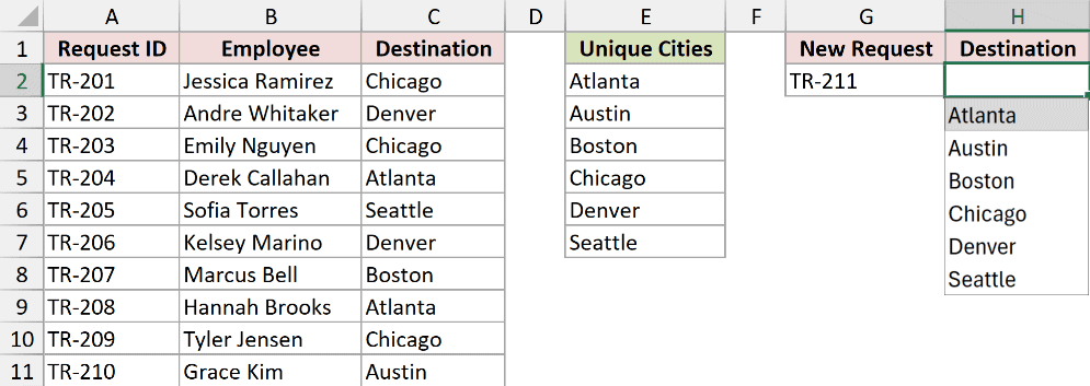
If you enter a new city within C2:C11, it appears automatically. If you extend the log below C11, extend the formula’s source range too.
Note: Keep the cells below E2 clear so Excel has room for the results. If another value blocks them, Excel returns #SPILL!, and the drop-down can’t use the list.
Create a Dependent Drop-Down List in Excel
A dependent drop-down changes its choices based on what you picked in another cell. Here, the City list will follow the Region you select.
Method #7: Using INDIRECT With Named Ranges
If each request row needs its own Region and City choice, you can name each group of cities. Excel can then match the selected Region to the right city list.
You can use this approach in older Excel versions as well as Microsoft 365.
Below I have travel requests in A1:D11 on the Dependent INDIRECT sheet. I keep three regional city lists in F1:H4.
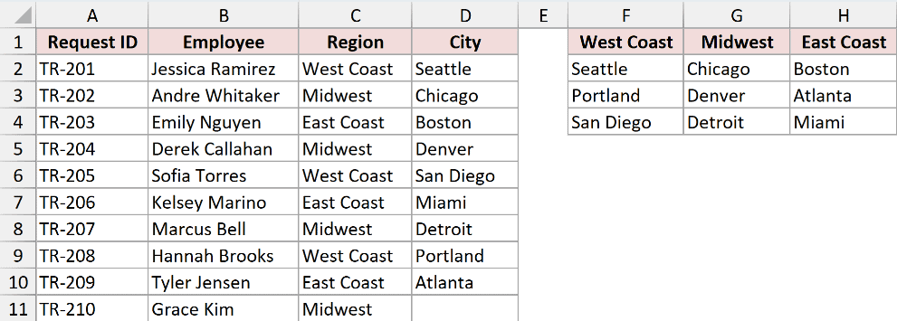
The request columns are Request ID, Employee, Region, and City. I arranged the source lists under West Coast, Midwest, and East Coast.
- In F2:F4, I have Seattle, Portland, and San Diego.
- In G2:G4, I have Chicago, Denver, and Detroit.
- In H2:H4, I have Boston, Atlanta, and Miami.
In row 11, Grace Kim’s request has Midwest selected and the City cell is blank. I want that cell to offer only the Midwest cities.
Here’s how to connect the two drop-downs:
- Select F1:H4. Go to Formulas > Create from Selection, check Top row, uncheck Left column, and click OK.
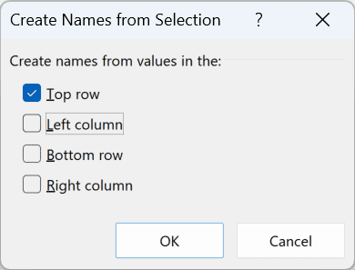
Excel creates West_Coast, Midwest, and East_Coast as the range names. It replaces each space in the headings with an underscore.
- Select C2:C11 and open Data tab > Data Validation. Choose List under Allow, enter
=$F$1:$H$1in Source, and click OK.
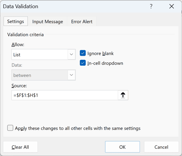
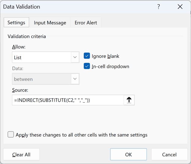
- Select D2:D11 with D2 as the active cell. Open Data tab > Data Validation, choose List under Allow, enter the following formula in Source, and click OK.
=INDIRECT(SUBSTITUTE(C2," ","_"))
How does this formula work?
SUBSTITUTE changes the spaces in the Region entry to underscores. With West Coast, it returns West_Coast, which matches the range name.
INDIRECT tells Excel to treat that text as a cell range. Data Validation then uses the cities from that range as your choices.
Because C2 is a relative reference, each row checks its own Region cell. That’s why you need D2 active when you apply the rule to D2:D11.
Now when you open Grace Kim’s City drop-down in row 11, you’ll see Chicago, Denver, and Detroit because her Region is Midwest.
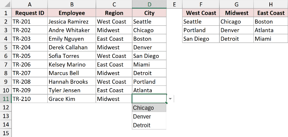
Note: When you change a Region, Excel updates the available cities but doesn’t clear the selected City. Choose the City again after you change the Region.
Method #8: Using the FILTER Function (Microsoft 365)
If you only need one entry card, FILTER can build the City choices from the Region you select. You won’t need to name a separate city range for each region.
You can use this method in Microsoft 365 and Excel 2021 or later.
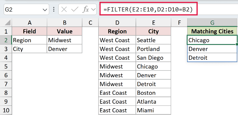
Below I have a Field and Value card in A1:B3 on the Dependent FILTER sheet. I keep the Region and City data in D1:E10.
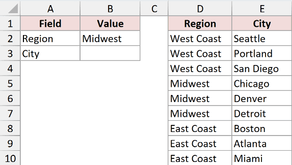
On the card, A2 is Region, B2 is Midwest, A3 is City, and B3 is Denver.
In D2:E10, I pair West Coast with Seattle, Portland, and San Diego; Midwest with Chicago, Denver, and Detroit; and East Coast with Boston, Atlanta, and Miami.
Here’s how to create the dependent list:
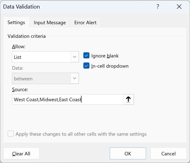
- Select B2 and open Data tab > Data Validation. Choose List under Allow, type
West Coast,Midwest,East Coastin Source, and click OK.
- Enter Matching Cities in G1. In G2, enter the following formula and press Enter.
=FILTER(E2:E10,D2:D10=B2)
How does this formula work?
D2:D10=B2 checks each source row against the Region selected in B2. With Midwest selected, the three Midwest rows match.
FILTER returns the matching cities from E2:E10. Excel fills the cells from G2 with Chicago, Denver, and Detroit.
- Select B3 and open Data tab > Data Validation. Choose List under Allow, enter
=$G$2#in Source, and click OK.
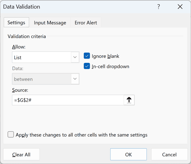
Now when you open the City drop-down, you’ll see Chicago, Denver, and Detroit. B3 contains Denver, which is one of those choices.
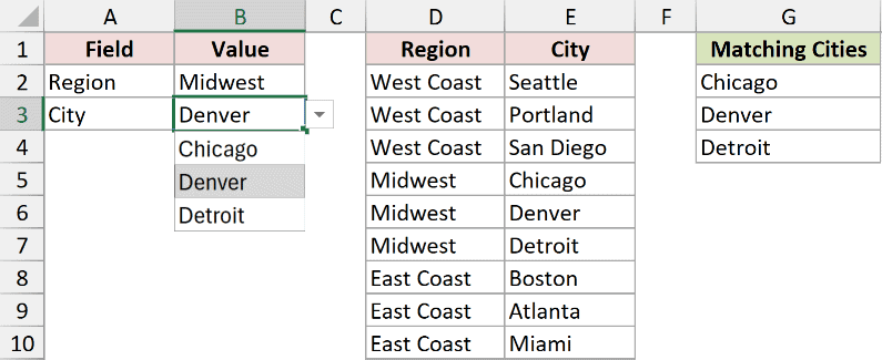
When you change B2, Excel recalculates the city list in G2. The # keeps the City drop-down connected to every returned city.
The formula only checks D2:D10 and E2:E10. If you add source rows, extend those references or Excel won’t search the new rows.
Note: Select a valid Region before you use the City list. When you change Regions, FILTER updates the choices but doesn’t replace the current value in B3.
Other Ways to Add a Drop-Down List in Excel
Data Validation will cover most drop-downs. But if it doesn’t fit your worksheet, the next methods let you choose an item in other ways.
Method #9: Using a Combo Box Form Control
A combo box is a drop-down control that sits over the worksheet instead of inside a cell. You can place it anywhere and resize it.
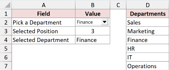
Below I have a Field and Value card in A1:B4 on the Combo Box sheet. I keep the Departments list in D1:D7.
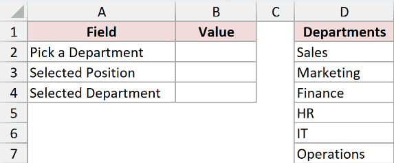
On the card, A2 says Pick a Department, A3 says Selected Position, and A4 says Selected Department. D2:D7 contains Sales, Marketing, Finance, HR, IT, and Operations.
I’ll place the combo box over B2. B3 will be the linked cell, which stores the selected item’s position. B4 will show the department name.
Here’s how to add the control:
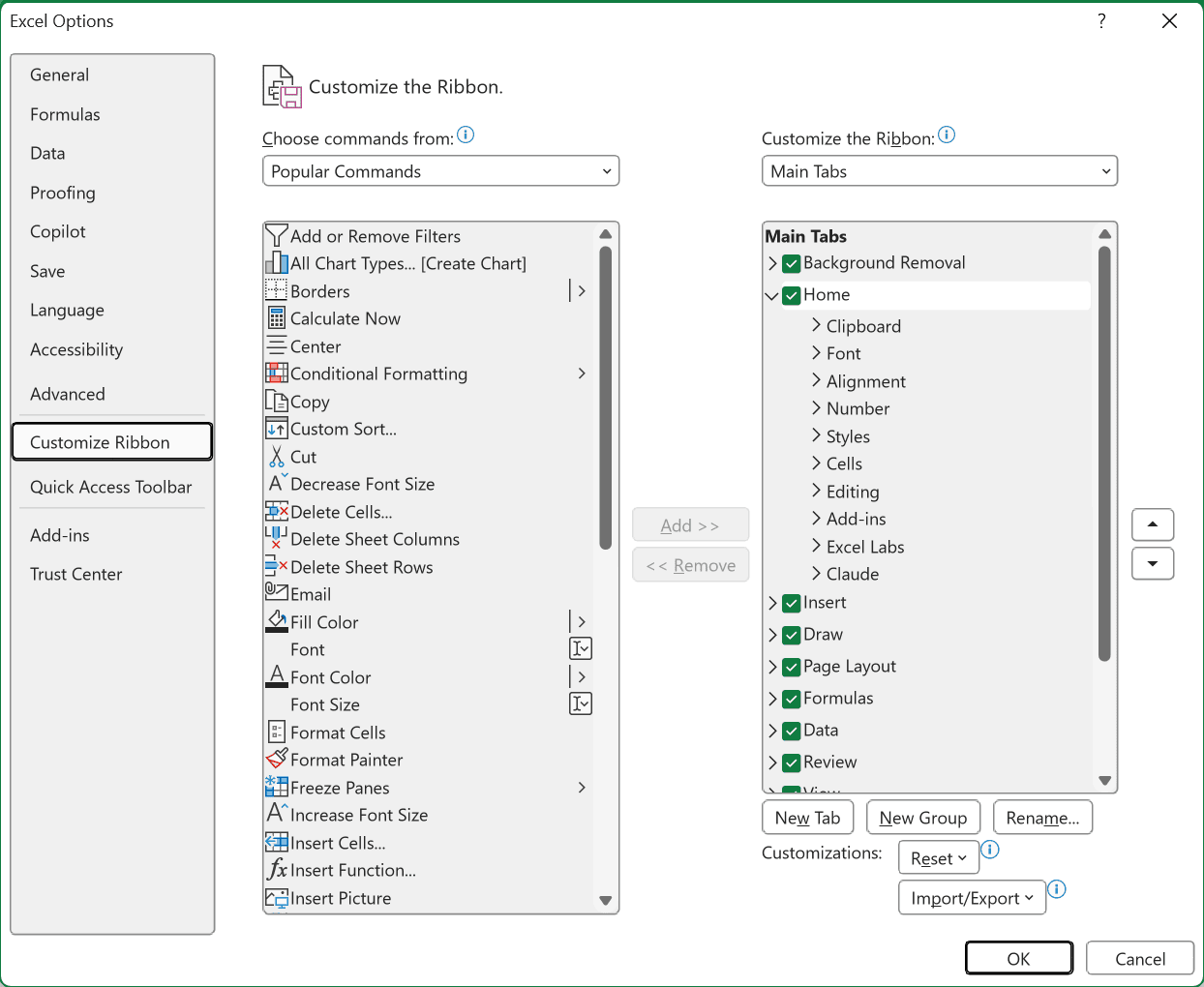
- Go to File > Options > Customize Ribbon. Check Developer in the main tabs list and click OK.
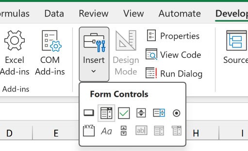
- Go to Developer > Insert > Form Controls > Combo Box, then draw the control over B2.
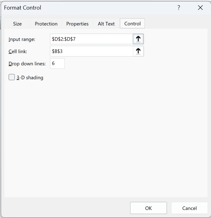
- Right-click the combo box and choose Format Control. On the Control tab, set Input range to
$D$2:$D$7, Cell link to$B$3, and Drop down lines to 6. Click OK.
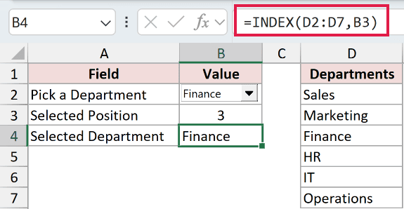
- Choose Finance in the combo box. Then enter the following formula in B4.
=INDEX(D2:D7,B3)
How does this formula work?
Finance is the third item in D2:D7, so the combo box puts 3 in B3. INDEX then returns the third value from that range.
Now the card shows 3 for Selected Position and Finance for Selected Department.
The formula returns one department because the combo box allows one selection. It doesn’t need to return a list of results.
You can resize the combo box by dragging its handles. Keep in mind that worksheet zoom also changes how large it looks.
Note: The Form Control sits over the worksheet instead of inside a cell. Its linked cell returns a position, so use the INDEX result when you need the department name.
Method #10: Using a VBA Macro
If you set up the same travel-mode list regularly, a short macro can add the drop-down to C2:C11 for you.
Below I have travel requests on the VBA Macro sheet. A1:C11 contains the Request ID, Employee, and Travel Mode columns, with C2:C11 blank.
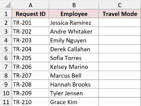
The macro works on whichever sheet is active, and it replaces any validation already in C2:C11. Make sure VBA Macro is active before you run it.
Here is the VBA code:
Sub AddTravelModeDropDown()
    With ActiveSheet.Range("C2:C11").Validation
        .Delete
        .Add Type:=xlValidateList, AlertStyle:=xlValidAlertStop, _
             Operator:=xlBetween, Formula1:="Flight,Train,Car,Bus"
        .IgnoreBlank = True
        .InCellDropdown = True
        .ShowError = True
    End With
End SubHere’s how to use the macro:
- With the VBA Macro sheet active, press Alt+F11 to open the Visual Basic Editor. Choose Insert > Module.
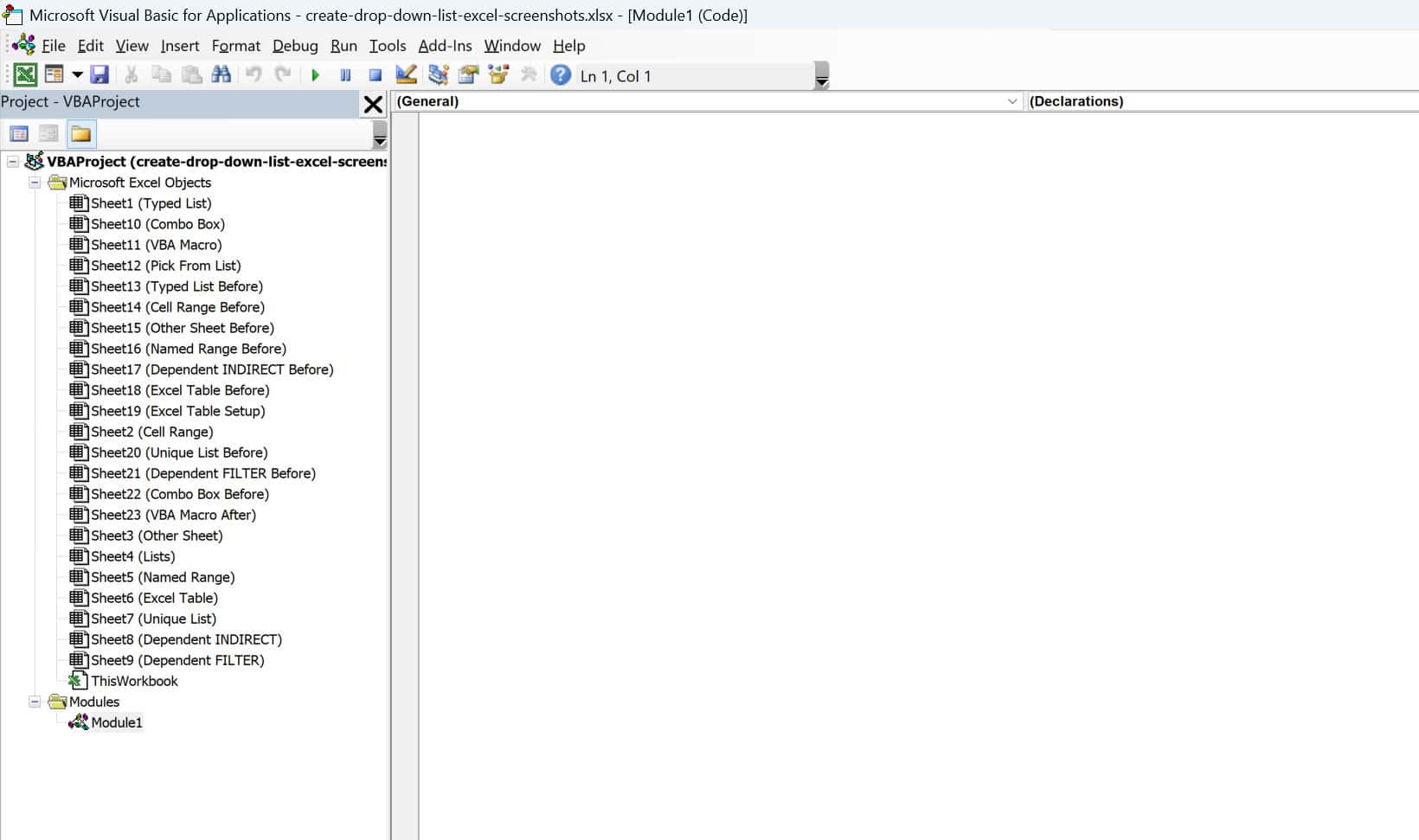
- Paste the code into the module. Place the cursor inside AddTravelModeDropDown and press F5 to run it.
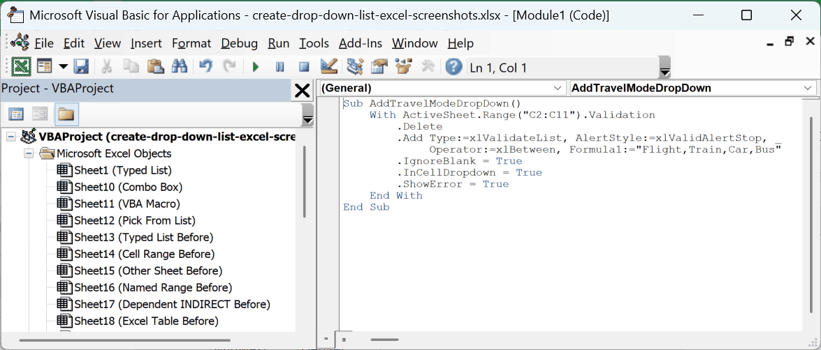
You can also run AddTravelModeDropDown from Excel with Alt+F8. Then return to the worksheet and use the list.
Now when you click any cell in C2:C11, you’ll see Flight, Train, Car, and Bus in the drop-down.
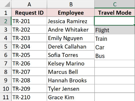
The code removes the old validation rule before adding the new List rule and its in-cell arrow. It doesn’t change the values already in C2:C11.
xlValidAlertStop and .ShowError = True tell Excel to show a Stop alert when someone types an entry that isn’t on the list.
Note: If you want to keep the macro, save the file as an Excel Macro-Enabled Workbook (.xlsm). You can run VBA in desktop Excel, but not Excel for the web.
Method #11: Using Pick From Drop-down List (No Setup)
If you need a quick choice from text already in the column, you can skip Data Validation entirely.
Below I have a request list on the Pick From List sheet. A1:C11 contains the Request ID, Employee, and Department columns, with C11 blank.
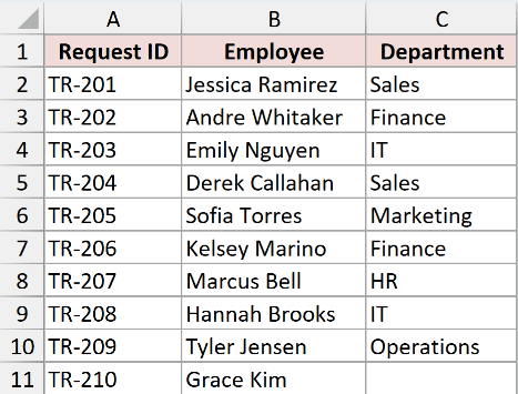
In C2:C10, I have Sales, Finance, IT, Sales, Marketing, Finance, HR, IT, and Operations.
Here’s how to reuse one of those departments:
- Select C11, right-click, and choose Pick From Drop-down List. You can also press Alt+Down.
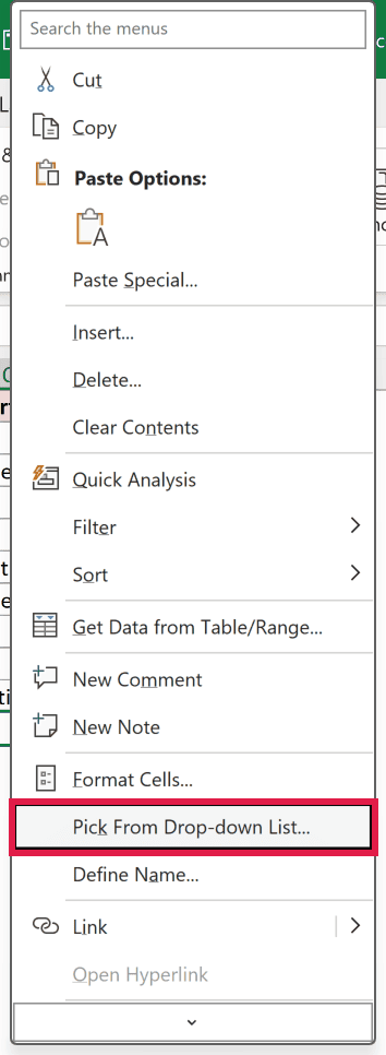
When you open the list, Excel shows Finance, HR, IT, Marketing, Operations, and Sales in order without duplicates. Choose the department you want in C11.
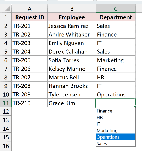
I use this when I’m continuing a column and don’t want to retype an entry that’s already there.
Note: Pick From Drop-down List doesn’t create a validation rule or block other entries. It only shows text that’s already in the column.
Which Drop-Down Method Should You Use?
If you’re not sure which method fits your worksheet, use this table to compare all 11 options.
| Method | Updates automatically? | Excel version | Best for |
|---|---|---|---|
| 1. Typed items | No; edit the rule | All desktop versions | A short, fixed list |
| 2. Cell range | Edits within the range | All desktop versions | Choices stored beside your data |
| 3. Another sheet | Edits within the range | Excel 2010 onwards | Keeping source lists separate |
| 4. Named range | Edits within the named range | All desktop versions | Reusing an easy-to-read source |
| 5. Excel Table | Yes, when the table expands | Excel 2007 onwards | A growing list; my recommendation |
| 6. UNIQUE and spill reference | Yes, within the formula’s source | Microsoft 365 / Excel 2021+ | Sorted choices without duplicates |
| 7. INDIRECT and named ranges | Yes, when the region changes | All desktop versions | Dependent choices across request rows |
| 8. FILTER | Yes, when the region or source data changes | Microsoft 365 / Excel 2021+ | A dependent entry card |
| 9. Combo Box Form Control | Edits within the input range | Desktop Excel | A separate, resizable selector |
| 10. VBA macro | No; rerun with revised items | Desktop Excel with VBA | Repeating the same setup |
| 11. Pick From Drop-down List | Yes, from existing column entries | Desktop Excel | Quickly reusing text without setup |
Additional Notes About Creating Drop-Down Lists in Excel
- To copy a drop-down, copy its cell, select the destination cells, and use Paste Special > Validation. You can also use the fill handle, but it may copy values or a series too.
- If you want to guide someone through the entry, use Input Message to show instructions when they select the cell. Error Alert controls what happens when they type an invalid entry.
- Choose Stop when you need to block invalid typed entries. Warning and Information allow them after a prompt. Pasting can bypass validation, so the rule can’t fully check imported entries.
- If your Microsoft 365 version includes drop-down AutoComplete, type in the cell to filter the choices. Excel can match text from anywhere in an item.
- On Windows, Alt+Down opens the selected cell’s drop-down. On a Mac, use Data > Data Validation, and use Cmd instead of Ctrl for common editing shortcuts.
- A standard Data Validation drop-down shows eight items before you need to scroll. You can’t change its font or font size, but you can resize a combo box.
Frequently Asked Questions
How Do I Edit or Add Items to a Drop-Down List?
Select a cell with the drop-down and open Data tab > Data Validation. Look at the Source box to see where the items come from.
If you typed the choices directly into the Source box, edit them there. If the drop-down uses cells or a named range, edit those cells and extend its reference if needed.
If the list uses a table, add the item directly beneath that table. Your new choices won’t replace values that you’ve already selected in other cells.
Can a Drop-Down List Allow Multiple Selections?
You can make one selection per cell with a standard Data Validation drop-down. If you choose another item, Excel replaces the previous one.
If you want to keep several selections in one cell, you’ll need extra automation, such as a worksheet event macro.
How Do I Remove a Drop-Down List?
Select the cells containing the list. Go to Data tab > Data Validation, click Clear All in the dialog, then click OK.
This removes the validation rule but keeps the current values. If you press Delete on the worksheet, you’ll clear the values and leave the drop-down rule in place.
Conclusion
For most lists, I recommend the Excel Table method because you can add another choice by typing beneath the source table.
When one choice depends on another, or you need to remove duplicates, I’d use the matching formula method instead.
But if you only need four fixed choices, type them into Data Validation and move on.
Other Excel articles you may also like:
