
If you’ve ever copied a formula into one cell and then retyped it row by row, the fill handle can do that in one drag. It’s the small square at the bottom-right corner of any selected cell.
Most people never notice it because nothing on the ribbon points to it, so they copy and paste instead. Once you know it’s there, filling formulas, numbers, dates, and custom lists takes seconds.
In this guide, I’ll show you six easy ways to use the fill handle in Excel.
Method #1: Copying a Formula Down a Column
The fill handle really shines when you’ve got a formula in one cell and want the same logic in every row below. It’s the method I reach for most, so let’s start here.
Below I’ve got a list of warehouse inventory items. Column C has the Qty for each item, and I want an In Stock or Reorder status in column D based on whether the Qty reaches at least 40.
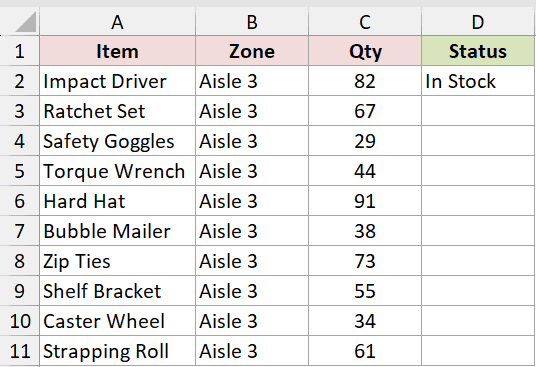
Type this formula in cell D2:
=IF(C2>=40,"In Stock","Reorder")
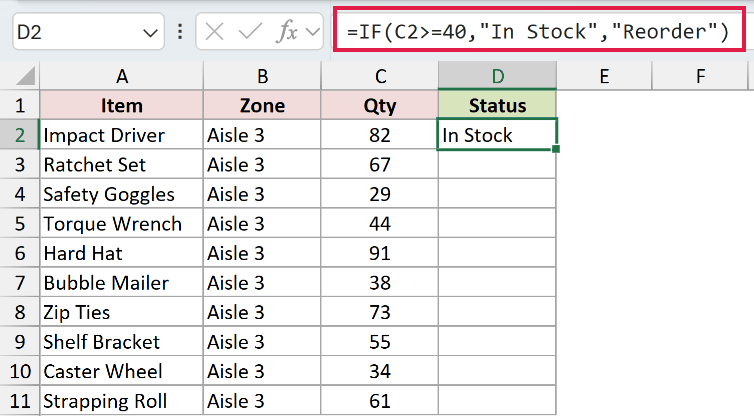
Now select D2, hover over the small square at its bottom-right corner until the cursor becomes a thin black plus sign, and double-click. Excel fills the formula down to the last row that has data beside it.
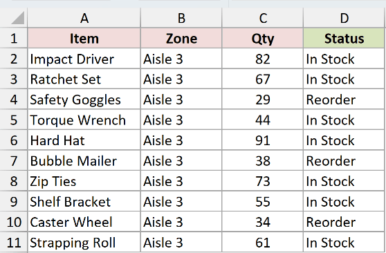
Note: You can also drag the fill handle down instead of double-clicking. Double-clicking is faster because it stops on its own at the end of the adjacent data.
How does this fill work?
When D2 holds =IF(C2>=40,"In Stock","Reorder"), the fill handle copies that pattern down. In D3 the reference becomes C3, in D4 it becomes C4, and so on.
These are relative references, so each row checks its own Qty. Impact Driver has a Qty of 82, so it gets In Stock. Safety Goggles sits at 29, so it gets Reorder.
Method #2: Creating a Series of Numbers
Here’s another handy use. The fill handle can build a run of numbers for you, which is great when you want to add item numbers or a serial column.
For the same items, I’ll number them from 1 to 10 in an Item No column.
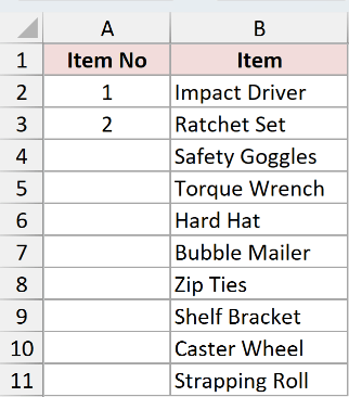
Here are the steps to fill a number series:
- Type 1 in the first cell and 2 in the cell right below it.
- Select both cells, then drag the fill handle down to the last row.
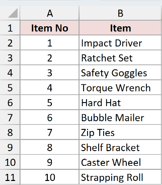
Excel reads the gap between 1 and 2 as a step of 1 and keeps going: 3, 4, 5, all the way to 10.
Note: If you type just one number and drag, Excel copies that same number to every cell. Entering two numbers first sets the step size, so 5 and 10 would fill 5, 10, 15, 20.
Method #3: Filling a Series of Dates
Dates work a little differently. With a date you only need one starting value, because Excel assumes you want to count up by one day each row.
I’ll add a Delivery Date column that starts from 01-Sep-2025.
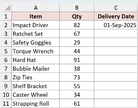
Here are the steps to fill a date series:
- Type 01-Sep-2025 in the first cell.
- Select that cell and drag the fill handle down.
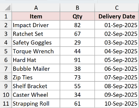
Excel fills 01-Sep-2025, 02-Sep-2025, 03-Sep-2025, and keeps going one day at a time.
Want to step by weekday, month, or year instead? Click the Auto Fill Options button that appears at the bottom-right after you drag.
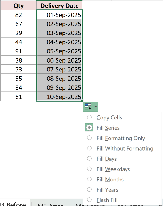
Pick Fill Months to jump to 01-Oct, 01-Nov, and so on, or Fill Weekdays to skip the weekends.
Method #4: Filling From a Custom List
Excel already knows a few lists, like Monday, Tuesday, Wednesday or January, February, March. You can teach it your own list too, so the fill handle cycles through it.
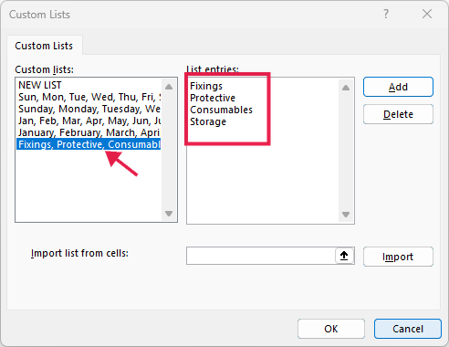
I often enter the same categories in the same order: Fixings, Protective, Consumables, Storage. Here’s how to save that as a custom list.
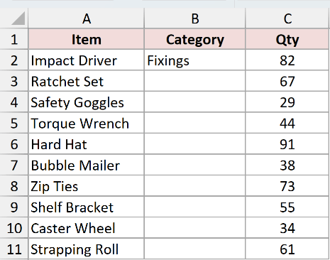
Here are the steps to set up a custom list:
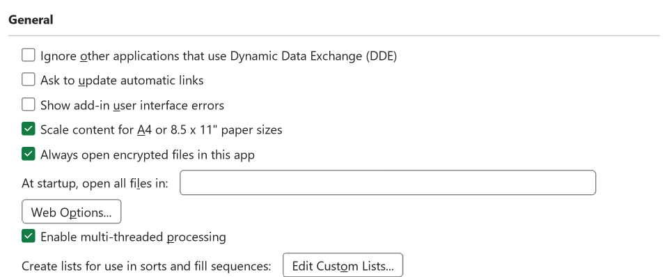
- In Windows, click File > Options > Advanced, scroll to the General section, and click Edit Custom Lists. On Mac, click Excel > Preferences > Custom Lists.
- In the List entries box, type each category on its own line, then click Add and OK.
- Type Fixings in a cell, select it, and drag the fill handle down.
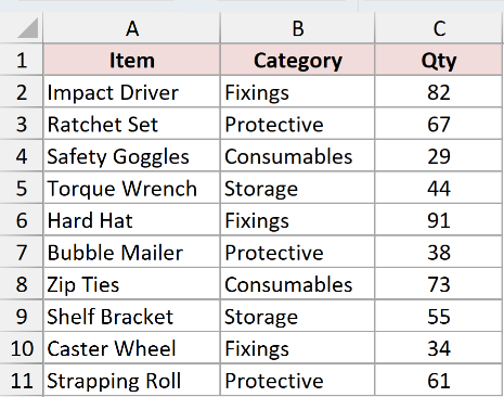
Excel fills Fixings, Protective, Consumables, Storage, then loops back to Fixings and repeats.
Method #5: Using Auto Fill Options (Fill Without Formatting)
Sometimes the cell you drag from has shading or a border you don’t want carried down. The Auto Fill Options button lets you fill just the values and leave the formatting behind.
In my inventory table, cell D2 has a light green fill. When I drag the formula down, that green comes along with it. Here’s how to drop it.
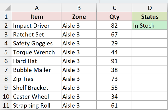
Here are the steps to fill without formatting:
- Drag the fill handle down as usual. You’ll see the green fill copied into the rows below.
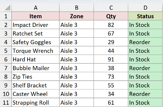
- Click the Auto Fill Options button at the bottom-right, then choose Fill Without Formatting.
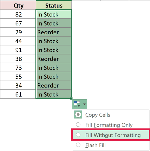
The formulas stay in place, but the green fill no longer copies down. Each row keeps whatever formatting it already had.
Method #6: Using the Ctrl + D Shortcut
Prefer the keyboard, or the fill handle is hidden? You can fill down without dragging at all. Ctrl + D copies the top cell of a selection into every cell below it.
Here I’ll copy the In Stock or Reorder formula from D2 down through D11 without touching the mouse.
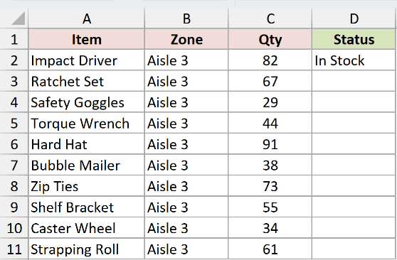
Here are the steps to fill down with the shortcut:
- Select the range that starts with the filled cell, so D2:D11.
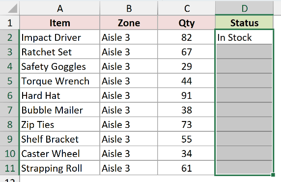
- Press Ctrl + D.
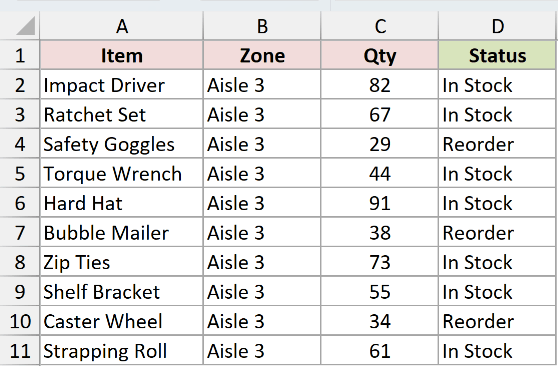
Excel copies D2 down the whole selection, adjusting the references just like the fill handle does. Ctrl + R does the same thing across to the right.
Note: Ctrl + D brings the formatting of the top cell along with the formula. To skip the formatting, copy the cell and use Paste Special > Formulas instead.
Additional Notes About the Fill Handle in Excel
- Right-click and drag the fill handle instead of left-clicking. When you let go, Excel shows a menu with options like Fill Series, Fill Formatting Only, and Fill Without Formatting.
- The fill handle carries formatting, borders, and conditional formatting along with the value, so watch for shading you didn’t mean to copy.
- You can drag in any direction, including up and to the left. For a series, dragging up or left continues it in reverse, counting backward.
- If a series suddenly won’t continue or the handle behaves oddly, that’s usually a settings or file issue rather than a technique problem. Our guide on why the Excel fill series is not working walks through the fixes.
Frequently Asked Questions
Why is my fill handle not showing up or not working in Excel?
The fill handle is the small square at the bottom-right of a selected cell.
If it’s missing in Windows, go to File > Options > Advanced and tick “Enable fill handle and cell drag-and-drop.” On Mac, go to Excel > Preferences > Edit and enable the fill handle option.
Also make sure you’ve clicked a cell first, since the square only appears on a selection.
How do I fill a series without changing the cell’s existing formatting?
Copy the source cell, select the target range, then use Home > Paste > Paste Special > Formulas. That brings the formula or value across without touching the formatting the target cells already have.
Can I create my own custom list for the fill handle to cycle through?
Yes. Besides typing a list by hand, you can turn a range you already have into a custom list.
Open File > Options > Advanced > Edit Custom Lists, click in the Import box, select the cells that hold your items, and click Import. The list is then available in every workbook.
Conclusion
The fill handle is one of those small Excel tools that saves you time every day once it becomes a habit.
For most work, copying a formula down a column (Method 1) is the one I reach for, with Ctrl + D as a quick keyboard backup. Give the custom list trick a try too if you type the same labels again and again.
Other Excel articles you may also like:
