
Excel’s T.INV.2T function returns the positive critical t value for a specified two-tailed probability and number of degrees of freedom.
Alpha is 1 minus the confidence level, so it is 0.05 for 95% confidence. The cutoff leaves that total probability across both tails.
You can use it for confidence intervals and two-tailed tests.
In this article, I’ll show you how to build a critical t table, calculate confidence intervals, and avoid the common alpha-halving mistake.
T.INV.2T Function Syntax in Excel
The function takes the total probability across both tails and the degrees of freedom.
=T.INV.2T(probability,deg_freedom)
- probability (required) is the total probability distributed across both tails of the Student’s t-distribution.
- deg_freedom (required) is the number of degrees of freedom for the distribution.
When to Use T.INV.2T Function
- Find the positive critical t value for a two-tailed statistical test.
- Build confidence intervals when the population standard deviation is unknown.
- Create a reusable critical t table for several confidence levels and sample sizes.
- Compare an absolute t statistic with its critical cutoff.
- Calculate margins of error for several groups with different sample sizes.
Example 1: Build a Critical t Table
Let’s start by replacing a printed critical t table with one formula.
Below is the dataset. Column A lists degrees of freedom, while columns B through D will hold critical values for three confidence levels.
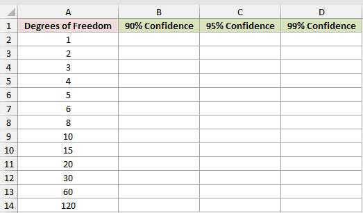
We want one formula to return every critical t value across the full table.
Here is the formula:
=T.INV.2T({0.1,0.05,0.01},A2:A14)
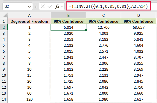
The array constant supplies the total two-tail alpha for the 90%, 95%, and 99% confidence columns. The range in column A supplies the degrees of freedom.
Excel combines the horizontal array with the vertical range, so the results spill across three columns and down all the listed rows.
At one degree of freedom, the three cutoffs are 6.314, 12.706, and 63.657. At 120 degrees of freedom, they fall to 1.658, 1.980, and 2.617.
Critical t values get smaller as degrees of freedom rise, but higher confidence levels still require larger cutoffs.
Pro Tip: This range formula spills in Excel 2021, Excel 2024, and Microsoft 365. Keep the output area empty, or Excel returns a #SPILL! error.
Example 2: Calculate a 95% Confidence Interval
This example builds a complete confidence interval from raw sample data.
Below is the dataset. Column A lists sample IDs LS-2041 through LS-2052, and column B holds the sodium readings.
The card in columns D and E holds the confidence setting and calculation cells.
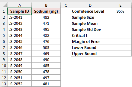
We want the sample statistics, critical t, margin of error, and both confidence limits.
First, count the sample measurements:
=COUNT(B2:B13)
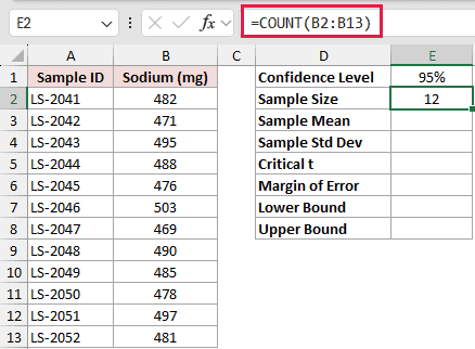
The COUNT formula returns a sample size of 12.
Next, calculate the sample mean:
=AVERAGE(B2:B13)
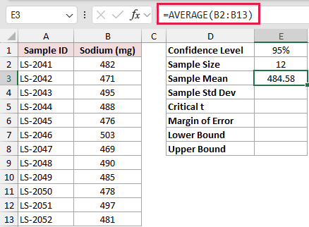
The average sodium measurement is 484.58 mg.
Now calculate the sample standard deviation:
=STDEV.S(B2:B13)
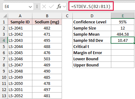
STDEV.S returns 10.47 for the spread of the sample measurements.
With those setup values ready, calculate the critical t:
=T.INV.2T(1-E1,E2-1)
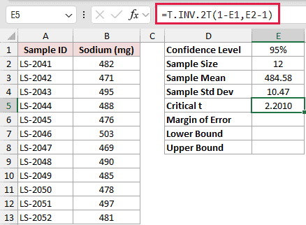
The expression 1-E1 converts the 95% confidence level to its total two-tail alpha. The expression E2-1 returns the degrees of freedom.
The resulting critical t is 2.2010.
Next, calculate the margin of error:
=E5*E4/SQRT(E2)
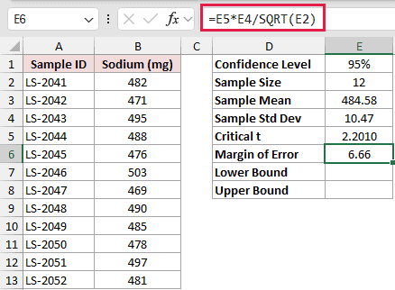
This multiplies the critical t by the sample standard deviation, then divides by the square root of the sample size. The margin is 6.66 mg.
Subtract that margin from the sample mean for the lower bound:
=E3-E6
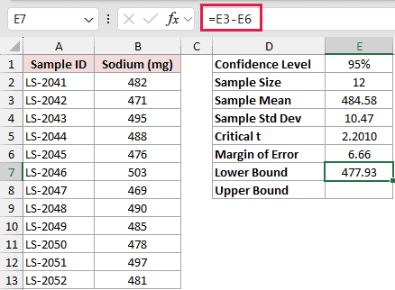
The lower confidence limit is 477.93 mg.
Add the margin to the sample mean for the upper bound:
=E3+E6
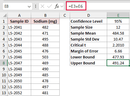
The upper confidence limit is 491.24 mg, so the interval runs from 477.93 mg to 491.24 mg.
CONFIDENCE.T can return the same 6.66 mg margin with =CONFIDENCE.T(1-E1,E4,E2). T.INV.2T is more useful when you also need to report the critical t value.
Example 3: Spill Margins Across Survey Groups
Here’s a practical way to calculate several margins of error at once.
Below is the dataset. Each row shows a location, response count, average rating, standard deviation, and empty columns for the critical t and margin.
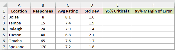
We want each location to use its own response count when calculating a 95% margin of error.
First, calculate a critical t for every row:
=T.INV.2T(0.05,B2:B7-1)
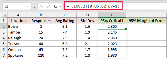
Subtracting one from each response count produces the degrees of freedom. The single formula spills six critical values down column E.
Boise has a critical t of 2.365 with 8 responses. Spokane has a smaller cutoff of 1.980 with 120 responses.
Now use those spilled critical values to calculate the margins:
=E2:E7*D2:D7/SQRT(B2:B7)
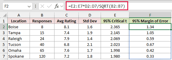
The formula multiplies each critical t by its standard deviation, then divides by the square root of that location’s response count.
The margins range from 1.34 for Boise to 0.33 for Spokane. More responses generally tighten the margin, but the standard deviation matters too.
Tucson’s margin is 0.67, while Raleigh’s is 0.59. Tucson has more responses, but its larger standard deviation keeps the margin wider.
Example 4: Test a t Statistic Against Its Cutoff
Here, critical t values become a clear testing decision.
Below is the dataset. It lists each lab balance, its reading count, its t statistic, and empty columns for the critical cutoff and decision.
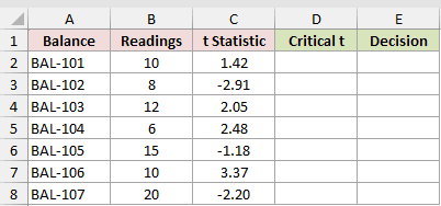
We want to flag balances whose absolute t statistic exceeds the correct two-tailed cutoff.
First, calculate the critical t for each balance:
=T.INV.2T(0.05,B2:B8-1)
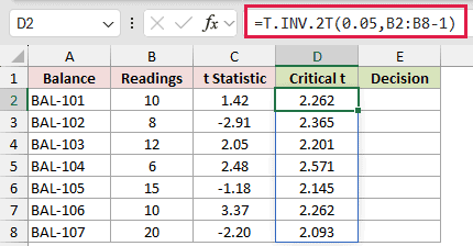
Different reading counts give different degrees-of-freedom values. The resulting cutoffs run from 2.093 to 2.571 in this dataset.
Now compare the size of each t statistic with its cutoff:
=IF(ABS(C2:C8)>D2:D8,"Significant bias","No significant bias")
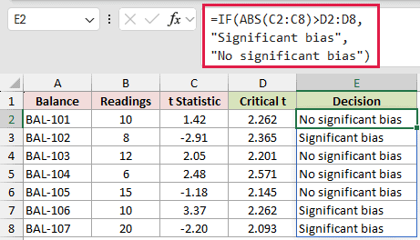
ABS makes negative and positive t statistics comparable by magnitude. Without it, a large negative statistic would never be greater than a positive cutoff.
BAL-102, BAL-106, and BAL-107 return Significant bias. The other four balances return No significant bias.
T.DIST.2T works in the opposite direction. It starts with the absolute t statistic and returns the two-tailed probability instead of the critical cutoff.
Pro Tip: A fixed z cutoff of 1.96 would wrongly flag BAL-103 and BAL-104 as biased. Their correct t cutoffs are 2.201 and 2.571, so neither clears the threshold.
Example 5: Use the Correct Two-Tail Probability
The last example clears up the most common T.INV.2T argument mistake.
Below is the parameter card. It contains alpha and degrees of freedom, plus labeled cells for the correct cutoff, a deliberate mistake, and two comparisons.
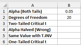
We want the two-tailed critical t for an alpha of 0.05 and 20 degrees of freedom.
Here is the correct formula:
=T.INV.2T(B1,B2)
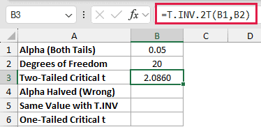
The result is 2.0860 because B1 already holds the total probability across both tails.
Here is the deliberate mistake labeled Alpha Halved (Wrong) in cell B4:
=T.INV.2T(B1/2,B2)
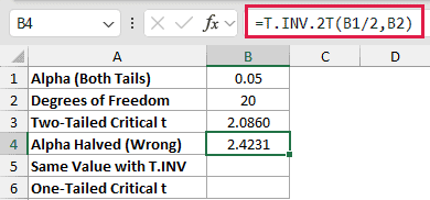
This wrongly halves alpha before passing it to a function that already expects both tails. The result rises to 2.4231 and is not the requested cutoff.
The equivalent T.INV formula handles one tail directly:
=T.INV(1-B1/2,B2)
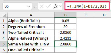
This formula returns the same 2.0860 value as the correct T.INV.2T formula.
For this one-tailed comparison, the row reuses B1’s 0.05 as a one-tail alpha. Doubling it passes 0.10 as the total two-tail probability:
=T.INV.2T(2*B1,B2)
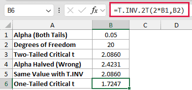
The result is 1.7247, the one-tailed critical t for alpha 0.05 and 20 degrees of freedom. It also equals =T.INV(1-B1,B2).
Pro Tip: Keep confidence level and alpha labels clear. If a cell stores 95% confidence, use 1-confidence_level. If it stores 0.05 alpha, pass that cell directly.
Tips & Common Mistakes
- A probability of 0 or less, or degrees of freedom below 1, returns
#NUM!. Keep probability between 0 and 1. Nonnumeric arguments return#VALUE!. Excel truncates 10.9 degrees of freedom to 10. - Excel 2019 and earlier do not support these dynamic spills, so enter separate formulas for the required rows and columns.
- T.INV.2T is not volatile. Its result changes only when the referenced inputs change.
- TINV is the legacy equivalent. Use T.INV.2T in new workbooks because its name makes the two-tailed behavior much clearer.
Check the label on your probability cell before you calculate. A 95% two-tailed confidence level needs 0.05, while a one-tailed alpha of 0.05 needs 0.10.
Then use the sample’s actual degrees of freedom instead of a fixed z cutoff.
Related Excel Functions / Articles:
