
The IMARGUMENT function in Excel returns the angle of a complex number in radians, measured from the positive real axis.
Think of a complex number as a point with a horizontal and vertical position. Its argument describes the direction to that point; its magnitude describes the distance.
In an electrical worksheet, the angle helps explain the phase relationship between voltage and current.
Comparing those phases takes care because subtracting their angles can give a misleading result.
IMARGUMENT Function Syntax in Excel
IMARGUMENT takes a complex number as its argument:
=IMARGUMENT(inumber)
- inumber (required): The complex number whose angle you want. Use a cell containing complex text, a real number, or the output of a function such as COMPLEX.
Complex text uses the form a+bi or a+bj, with a lowercase suffix. The result is a real number that you can format and use in calculations.
The angle is greater than -pi and less than or equal to pi radians. Zero has no defined direction, so it returns #DIV/0!.
When to Use IMARGUMENT Function
- Find the angle of a complex number while keeping its quadrant correct.
- Convert an impedance into a phase angle and interpret whether current leads or lags voltage.
- Calculate power factor directly from complex impedance.
- Combine an angle with a magnitude to display polar form.
- Find the phase difference between voltage and current readings.
Example 1: Find an Angle in Radians
Let’s start with points in different quadrants and on the axes.
Below is the dataset. Column A describes each position, column B holds the complex number, and column C is reserved for the angle in radians.
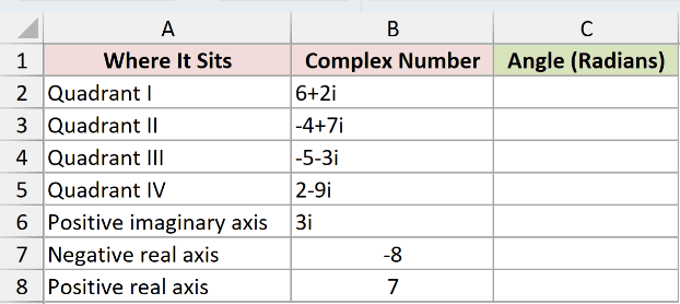
We want to calculate each point’s angle without losing its quadrant.
Enter this formula in C2 and copy it down through C8:
=IMARGUMENT(B2)
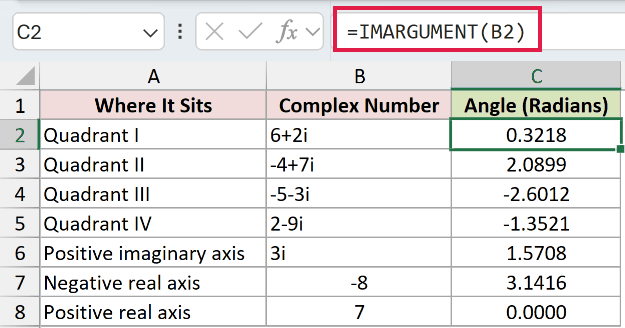
For 6+2i, C2 displays 0.3218 radians. The quadrant II point, -4+7i, returns 2.0899.
Below the real axis, the angles are negative. The quadrant III and IV rows display -2.6012 and -1.3521 respectively.
The negative real number in B7 returns 3.1416, the displayed approximation of pi. The positive real number in B8 returns 0.0000.
These are individual formulas copied down. Passing a bare range to IMARGUMENT returns a single #VALUE!, so filling down is the default approach throughout these examples.
Pro Tip: =IMARGUMENT(+B2:B8) uses unary plus to make the range spill. That approach works in Excel 2021, Excel 2024, and Microsoft 365.
In Excel 2019 and earlier, use the per-row formula shown above and fill down.
Example 2: Convert Impedance Angles to Degrees
Degrees make the phase relationship easier to read in an equipment list.
Below is the dataset. Columns A and B list office loads and their impedances. Columns C and D will hold phase angles and current-versus-voltage labels.
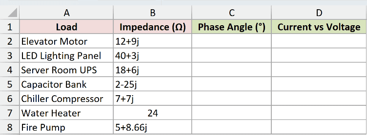
We want each impedance angle in degrees, followed by a label explaining its sign.
Enter this formula in C2 and copy it down through C8:
=DEGREES(IMARGUMENT(B2))
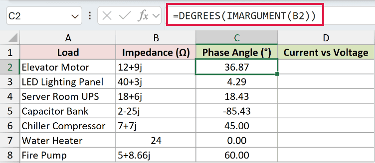
IMARGUMENT calculates the radians, then DEGREES converts them. The Elevator Motor returns 36.87 degrees, while the Capacitor Bank returns -85.43 degrees.
For these impedances, a positive angle means current lags voltage. A negative angle means current leads voltage, and a zero angle means they’re in phase.
To add those labels, enter this formula in D2 and copy it down through D8:
=IF(C2>0,"Lags voltage",IF(C2<0,"Leads voltage","In phase"))
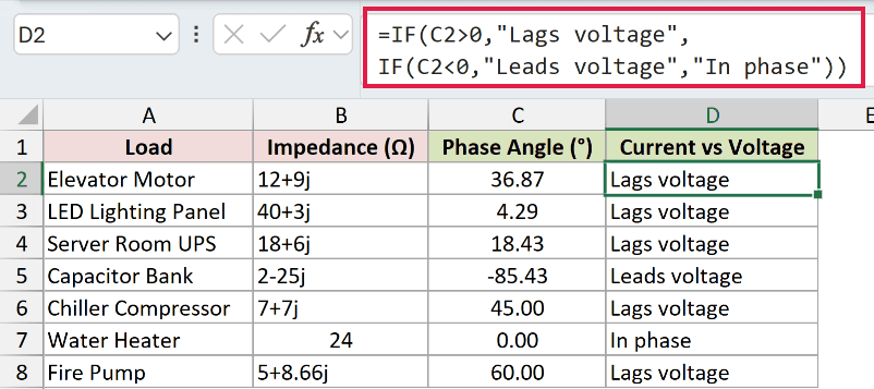
The Elevator Motor reads Lags voltage, the Capacitor Bank reads Leads voltage, and the Water Heater reads In phase beside its 0.00 angle.
The nested IF checks positive first, negative next, and uses the remaining case for an in-phase load.
Example 3: Calculate Power Factor From Impedance
You can also use the angle directly in a power factor calculation.
Below is the dataset. Columns A and B contain plant machines and impedances. The Power Factor and Needs Correction? columns hold the results.
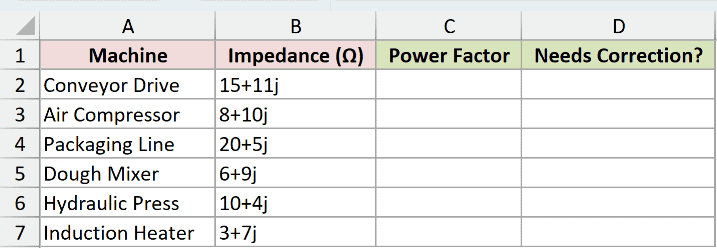
We want to calculate each machine’s power factor and flag those below the example’s chosen cutoff.
Enter this formula in C2 and copy it down through C7:
=COS(IMARGUMENT(B2))
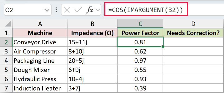
COS takes the radians returned by IMARGUMENT directly, so you can skip the conversion to degrees.
The Conveyor Drive displays 0.81, while the Packaging Line displays 0.97. These are numeric results, so the next formula can compare them directly.
Enter this flag formula in D2 and copy it down through D7:
=IF(C2<0.9,"Yes","No")
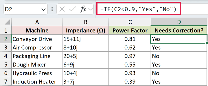
The Conveyor Drive returns Yes, and the Packaging Line returns No. Choose a cutoff that fits your worksheet.
Pro Tip: Keep the IMARGUMENT result in radians when feeding it into COS or SIN. Convert to degrees when you want a degree-based display, as in the previous example.
Example 4: Why ATAN Gets Quadrants Wrong
Dividing the imaginary part by the real part looks tempting, but that ratio loses information about the original point.
Below is the dataset. Columns A and B identify complex points. Columns C and E hold valid methods; column D is reserved for the incorrect ATAN approach.
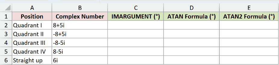
We want to compare the correct angles with the ATAN mistake and an ATAN2 check.
Start with IMARGUMENT in C2 and copy it down through C6:
=DEGREES(IMARGUMENT(B2))
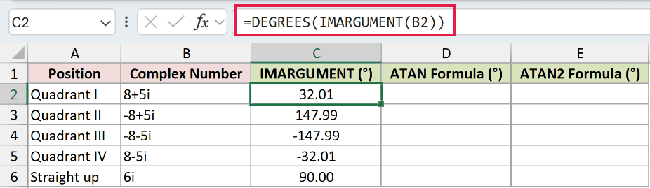
The quadrant II point returns 147.99 degrees, and the quadrant III point returns -147.99 degrees. The straight-up point returns 90.00 degrees.
For the deliberate mistake, enter this ATAN formula in D2 and copy it down through D6. This is what not to use:
=DEGREES(ATAN(IMAGINARY(B2)/IMREAL(B2)))
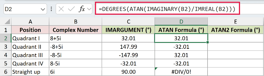
The incorrect ATAN column displays -32.01 for quadrant II and 32.01 for quadrant III. Both point to the wrong quadrant.
The same incorrect approach returns #DIV/0! for 6i in D6 because it divides by a zero real part. This is a deliberate error demonstration.
ATAN2 keeps the parts separate. Enter this comparison formula in E2 and copy it down through E6:
=DEGREES(ATAN2(IMREAL(B2),IMAGINARY(B2)))
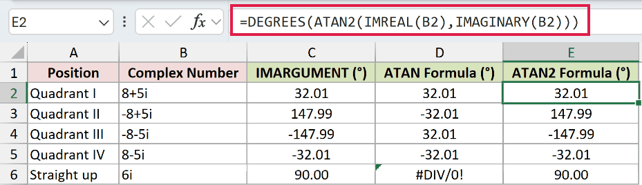
The ATAN2 comparison matches IMARGUMENT throughout, including 147.99, -147.99, and 90.00 for the rows where the ATAN mistake fails.
Excel’s ATAN2 takes the real part first and the imaginary part second. IMARGUMENT is shorter when you already have a complex number in a cell.
Example 5: Display Current in Polar Form
Polar form puts the magnitude and angle together in a readable label.
Below is the dataset. Columns A and B list equipment and complex current readings. Columns C, D, and E are prepared for magnitude, angle, and polar form.
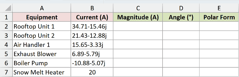
We want to show each current as a magnitude followed by its angle in degrees.
Calculate the magnitude in C2, then copy down through C7:
=IMABS(B2)
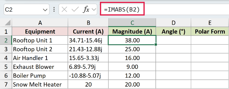
For Rooftop Unit 1, the magnitude displays as 38.00 amperes.
Calculate the angle in D2, then copy down through D7:
=DEGREES(IMARGUMENT(B2))
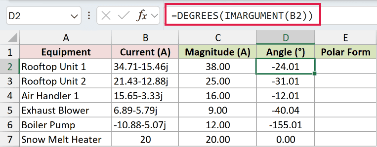
The angle displays as -24.01 degrees. These readings were rounded to two decimal places, so their calculated angles can land slightly away from round numbers.
Join the results in E2, then copy down through E7:
=TEXT(C2,"0.0")&" ∠ "&TEXT(D2,"0.0")&"°"
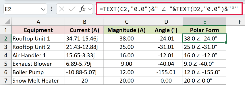
E2 displays 38.0 ∠ -24.0°. The Boiler Pump displays 12.0 ∠ -155.0°, preserving the negative angle for its quadrant.
How this formula works:
- Each TEXT function formats its numeric input using the pattern shown in the formula.
- The ampersands join the formatted magnitude, angle symbol, formatted angle, and degree symbol.
- The final label is text. Keep columns C and D for further numeric calculations.
Example 6: Avoid Phase-Difference Wrap-Around
Subtracting angles can produce a misleading phase difference when the readings sit on opposite sides of the negative real axis.
Below is the dataset. Store meters have voltage and current readings in B and C. Column D holds the subtraction mistake; E holds the corrected angle.
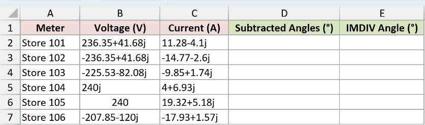
We want the voltage-minus-current phase difference within IMARGUMENT’s principal angle range.
First, demonstrate the subtraction mistake in D2 and copy it down through D7:
=DEGREES(IMARGUMENT(B2)-IMARGUMENT(C2))
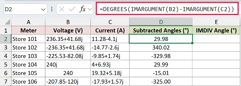
Store 101 displays 29.98 degrees in the subtraction column, but Store 102 displays 340.02 and Store 103 displays -329.98.
Those last values fall outside the intended range above -180 through +180 degrees. Each input angle is within range, but subtracting them doesn’t preserve that limit.
Use the corrected formula in E2 and copy it down through E7:
=DEGREES(IMARGUMENT(IMDIV(B2,C2)))
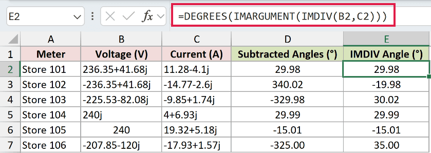
Store 102 now displays -19.98 degrees, and Store 103 displays 30.02 degrees. Store 106 returns 35.00, correcting the subtraction mistake’s -325.00.
IMDIV divides voltage by current first. IMARGUMENT then returns the quotient’s principal angle, keeping the phase difference within its defined range.
The phasor parts were rounded to two decimal places, which explains why some angles are a few hundredths away from round numbers.
Example 7: Handle Zero Without Hiding Errors
A missing harmonic current has no phase angle to calculate.
Below is the dataset. Columns A and B list harmonics and currents, including zero readings. Column C is the unguarded demonstration; D is the guarded result column.
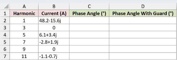
We want to show an angle for nonzero currents and a clear label when no angle exists.
Enter this unguarded formula in C2 and copy it down through C7 to demonstrate the zero-input error:
=DEGREES(IMARGUMENT(B2))
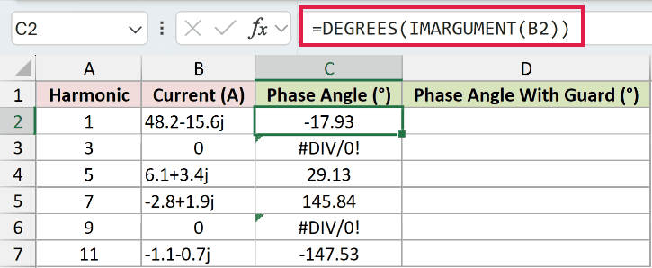
The unguarded demonstration returns -17.93 degrees in C2, but C3 and C6 deliberately show #DIV/0!. Both corresponding currents are zero.
Add a specific zero guard in D2 and copy it down through D7:
=IF(IMABS(B2)=0,"None",DEGREES(IMARGUMENT(B2)))
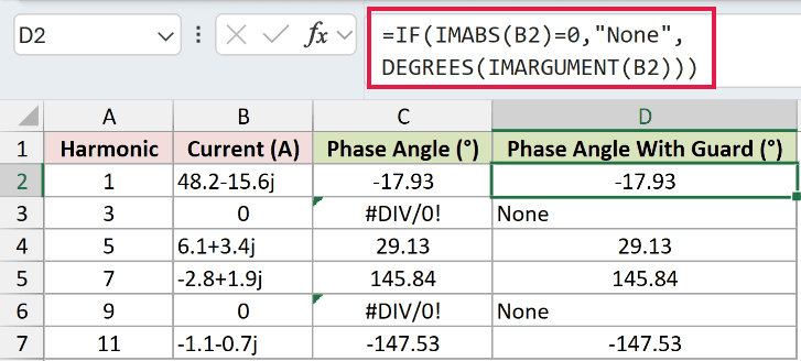
The guarded cells D3 and D6 display None. The nonzero reading in D2 still returns -17.93 degrees.
IMABS checks the current’s magnitude. IF returns the label when that magnitude is zero and calculates the angle otherwise.
Pro Tip: A specific zero guard preserves useful error messages from invalid complex inputs. IFERROR would hide those errors too, making a typo harder to distinguish from an absent current.
Tips & Common Mistakes
- Keep track of units. IMARGUMENT returns radians. Use DEGREES for a degree-based display, and leave the angle in radians for COS or SIN.
- Check the suffix. Complex inputs use lowercase
iorj. A capitalIreturns#NUM!. - Expect a sign change near the negative real axis. Crossing that axis can move the result from near positive pi to near negative pi.
- Use a nonnegative angle when needed. Apply MOD after converting to degrees for a 0-360 range. The ATAN2 article linked in Example 4 explains this normalization.
- Use the right function for the job. IMABS returns magnitude, IMARGUMENT returns angle, and COMPLEX builds complex text from separate real and imaginary parts.
- Don’t assume range support. A bare range returns
#VALUE!. The examples use per-row formulas copied down so each input is evaluated separately.
IMARGUMENT gives complex readings an angle you can use in your worksheet. Taking the quotient first keeps phase comparisons within the function’s angle range.
Related Excel Functions / Articles:
