
The IMAGINARY function in Excel returns the imaginary part of a complex number as a regular number, keeping its positive or negative sign.
In the notation a+bi, it extracts b. The result doesn’t include the i suffix, so you can use it in ordinary calculations.
For electrical power stored as complex text, that imaginary part represents reactive power. Extracting it lets you total the readings or classify loads by their sign.
I’ll show you how to summarize complex power, spot input problems, and count non-real roots with a range formula.
IMAGINARY Function Syntax in Excel
IMAGINARY takes a complex number as its required argument:
=IMAGINARY(inumber)
- inumber (required): The complex number to read, usually text in
a+biora+bjform. You can reference a cell or put complex text inside double quotes.
Use lowercase i or j as the suffix. IMAGINARY returns the signed coefficient as a number, while IMREAL extracts the real part.
When to Use IMAGINARY Function
- Extract imaginary coefficients from a column of complex numbers.
- Separate complex power into real and reactive numeric columns for totals.
- Classify electrical loads using the sign of their reactive power.
- Identify listed equation roots that have a nonzero imaginary part.
Example 1: Extract the Imaginary Part
Let’s start with a column containing different forms of complex numbers.
Below is the dataset. Column A contains complex numbers, and column B has the Imaginary Part header and cells for the results.
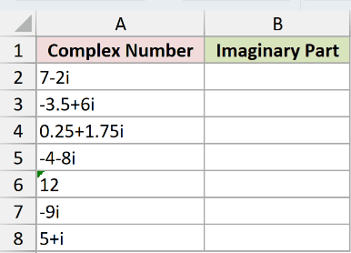
We want to extract each imaginary coefficient while keeping its sign and decimal value.
Enter this formula in B2, then copy it down through B8:
=IMAGINARY(A2)
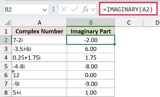
For 7-2i, B2 displays -2.00. The minus sign belongs to the imaginary coefficient, so it stays in the result.
The input 0.25+1.75i returns 1.75, while the pure imaginary value -9i returns -9.00.
The real-only input 12 returns 0.00. For 5+i, the coefficient is implied, and Excel displays 1.00.
These are numeric results. The decimal formatting in column B controls their appearance without turning them into complex text.
Pro Tip: Use a cell reference and copy down for ordinary lists. A bare range passed to IMAGINARY returns a single #VALUE!. Example 5 shows the extra step needed to spill.
Example 2: Split and Total Complex Power
Now let’s turn complex power readings into columns you can total.
Below is the dataset. Columns A and B list panels and complex power readings; columns C and D have result headers, with a Total row beneath them.
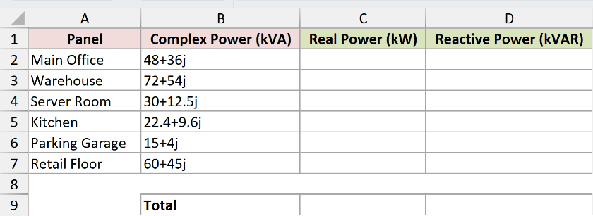
We want each panel’s real and reactive power as numbers, followed by separate totals.
In complex power notation S = P + jQ, P is real power in kW and Q is reactive power in kVAR.
First, enter the IMREAL formula in C2 and copy it down through C7:
=IMREAL(B2)
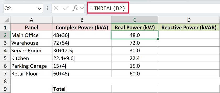
Main Office’s 48+36j reading returns 48.0 kW in C2.
Next, enter the IMAGINARY formula in D2 and copy it down through D7:
=IMAGINARY(B2)
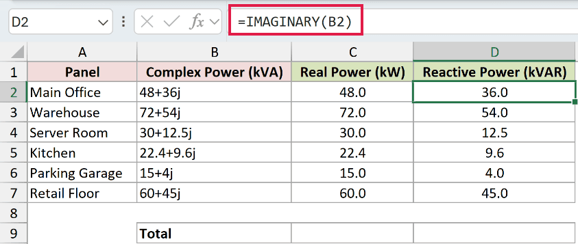
D2 returns 36.0 kVAR for Main Office. For Server Room, D4 returns 12.5 kVAR from 30+12.5j.
To total real power, enter this formula in C9:
=SUM(C2:C7)
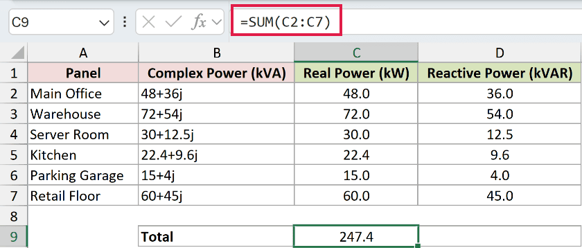
The real power total is 247.4 kW.
To total reactive power, enter this formula in D9:
=SUM(D2:D7)
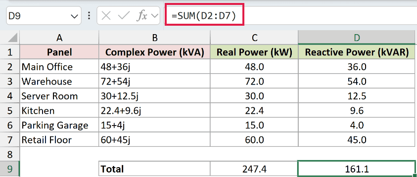
The reactive power total is 161.1 kVAR. SUM works directly because IMAGINARY has already converted the imaginary coefficients into numbers.
Example 3: Classify Loads by Reactive Power
The sign of reactive power can also tell you what kind of load you’re looking at.
Below is the dataset. Columns A and B contain equipment names and complex power; columns C and D are reserved for reactive power and load type.
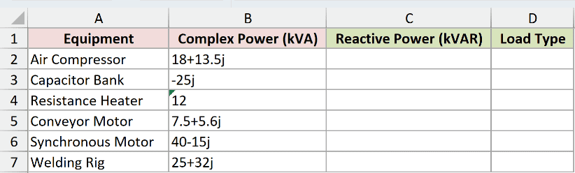
We want to label each load as lagging, leading, or resistive using its reactive power.
Enter this formula in C2 and copy it down through C7:
=IMAGINARY(B2)
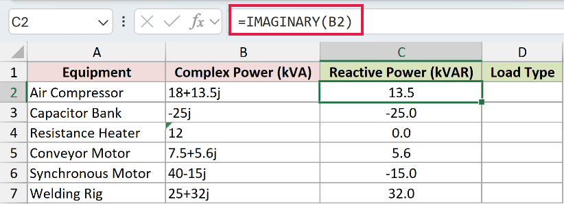
Air Compressor returns 13.5 kVAR, Capacitor Bank returns -25.0 kVAR, and Resistance Heater returns 0.0 kVAR.
Under the S = P + jQ convention, positive reactive power indicates a lagging, inductive load. Negative reactive power indicates a leading, capacitive load.
Enter this classification formula in D2, then copy it down through D7:
=IF(C2>0,"Lagging (inductive)",IF(C2<0,"Leading (capacitive)","Resistive"))
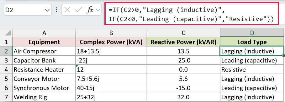
How this formula works:
- The first IF checks whether reactive power is positive and returns Lagging (inductive), as it does for Air Compressor.
- Otherwise, the nested IF checks for a negative value and returns Leading (capacitive), as it does for Capacitor Bank.
- When the reactive power is zero, it returns Resistive, as it does for Resistance Heater.
IMAGINARY provides the numeric value that IF tests. The classification comes from the sign of that value.
Example 4: Check Accepted Inputs and Errors
Some unusual-looking inputs work, while small changes to the suffix cause an error.
Below is the dataset. Column A labels each input type, column B contains the test inputs, and column C is reserved for IMAGINARY results.
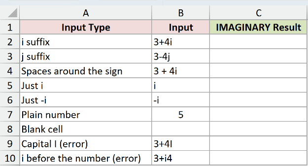
We want to distinguish accepted inputs, deliberate errors, and inputs that silently return zero.
Enter this formula in C2 and copy it down through C10:
=IMAGINARY(B2)
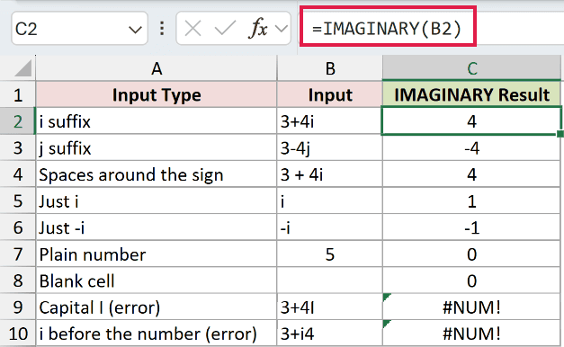
Lowercase suffixes and spaces around the sign work, but malformed complex text causes errors:
- Lowercase i:
3+4ireturns 4 in C2. - Lowercase j:
3-4jreturns -4 in C3. - Spaces around the sign:
3 + 4ireturns 4 in C4. Those spaces are tolerated. - Just i:
ireturns 1 in C5 because the coefficient is implied. - Just -i:
-ireturns -1 in C6. - Plain number: The numeric input
5silently returns 0 in C7 because it has no imaginary component. - Blank cell: Empty B8 silently returns 0 in C8. This zero can hide a missing reading.
- Capital I, deliberate error:
3+4Ireturns #NUM! in C9. Change the suffix to lowercase. - Suffix before its coefficient, deliberate error:
3+i4returns #NUM! in C10. Put the coefficient before the suffix.
The errors in C9 and C10 are intentional demonstrations. Their result styling doesn’t make those inputs valid.
Pro Tip: Check whether an input is missing before interpreting a zero result. IMAGINARY alone cannot distinguish a blank cell from a valid real-only value.
Example 5: Count Non-Real Roots With a Spill
A spilled column of imaginary parts lets you count non-real roots with one COUNTIF formula.
Below is the dataset. Columns A and B list equations and their first roots; column C has the Imaginary Part header, and E1 labels the count cell.
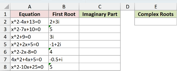
We want to count the listed roots whose imaginary part is nonzero. The roots are already supplied; this example doesn’t solve the equations.
Enter this formula in C2:
=IMAGINARY(+B2:B8)
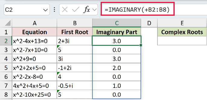
The unary plus makes Excel pass the range’s values as an array that IMAGINARY can process. Without that coercion, a bare range returns a single #VALUE!.
The formula spills into C2:C8, displaying 3.0, 0.0, 3.0, 2.0, 0.0, 1.0, 0.0.
This spill works in Excel 2021, Excel 2024, and Microsoft 365. In Excel 2019 and earlier, use the per-row method from Example 1 and fill down.
Now enter the count formula in E2:
=COUNTIF(C2:C8,"<>0")
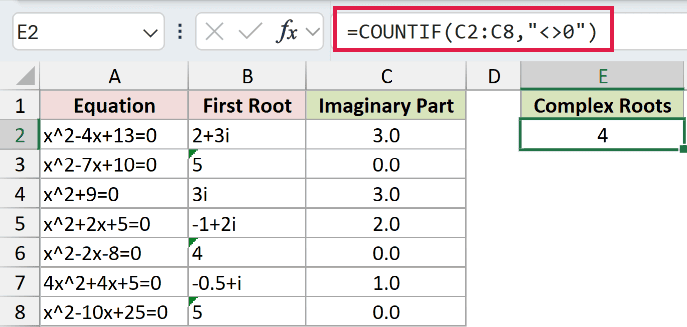
The result is 4. COUNTIF‘s "<>0" criterion counts the extracted values that aren’t zero.
Although the card says Complex Roots, it counts non-real roots listed in column B. It doesn’t count every root of every equation, since only the first root is shown.
Tips & Common Mistakes
- Keep the suffix lowercase. Use
iorj. A capitalIcauses #NUM!, as the deliberate error in Example 4 shows. - Preserve the sign. A negative imaginary coefficient can carry meaning, such as the leading load in Example 3. Don’t discard it when extracting the value.
- Treat missing inputs separately. A blank cell silently returns zero. Check the source before using that result to classify a reading.
- Don’t pass a bare range. Use the per-row approach or the explained unary-plus spill in Example 5.
- Choose the component you need. IMREAL extracts the real part; IMAGINARY extracts the imaginary coefficient. IMABS returns the magnitude as a number. COMPLEX builds complex text from separate parts.
- Extract before rounding. For a complex quotient returned by IMDIV, use IMAGINARY to extract the imaginary coefficient as a number before rounding it.
Once the imaginary part is numeric, use ordinary worksheet functions for totals and decisions. Keep the original complex text alongside it so you can trace each result.
Related Excel Functions / Articles:
