
Excel’s SUM function adds numbers from values, cell references, or ranges and returns their total.
You can add up a bunch of numbers across one column, separate ranges, or corresponding cells on multiple sheets. Text within referenced ranges is ignored.
In this article, I’ll show you how to add separate ranges, total matching rows, and sum the same cell across worksheets.
SUM Function Syntax in Excel
Here is what the SUM function looks like:
=SUM(number1, [number2], ...)
- number1 = the first number, cell, or range to add.
- number2… = optional additional numbers, cells, or ranges.
You can mix single cells and ranges in the same formula, and SUM ignores any text or blank cells.
When to Use the SUM Function
- Adding up a column or row of numbers, like sales, hours, or expenses.
- Totaling several separate ranges in one formula instead of many.
- Getting a clean total even when the data has stray text or blanks.
- Rolling up the same cell from monthly tabs into one quarter total.
- Building quick running totals or grand totals at the bottom of a report.
Example 1: Add Up a Range of Numbers
Let us start with the most common job, totaling a single column.
Here we have months in column A and their sales figures in column B, ten rows in total.
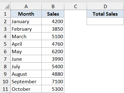
You want to add up the sales for all ten months.
Here is the formula:
=SUM(B2:B11)
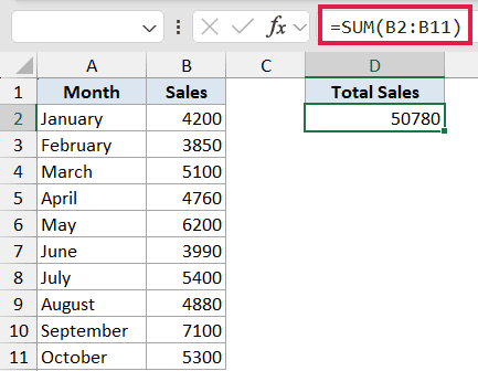
Point SUM at a single range and it adds everything inside it, returning 50780 here.
One nice bonus: SUM auto-adjusts if you insert or delete rows inside the range, so your total stays correct without editing the formula.
Pro Tip: Select the cell right below your numbers and press Alt and = together (AutoSum). Excel writes the SUM formula and picks the range for you.
Example 2: Sum More Than One Range at Once
SUM is not limited to one block of cells. You can hand it several ranges in the same formula.
Here we have regions in column A, with Q1 sales in column B and Q2 sales in column C, across five rows.
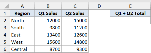
You want to add up both quarters across every region in a single formula.
Here is the formula:
=SUM(B2:B6,C2:C6)
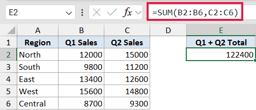
Separate each range or cell with a comma and SUM adds them all together, giving 122400.
You can mix ranges and individual cells the same way, like =SUM(B2:B6, C2, 100), and SUM still totals everything you list.
Example 3: SUM Ignores Text and Blanks
Real data is rarely clean. SUM handles messy columns better than you might expect.
Here we have items in column A and a Value column in column B, ten rows, where the values include some text entries and a blank cell.
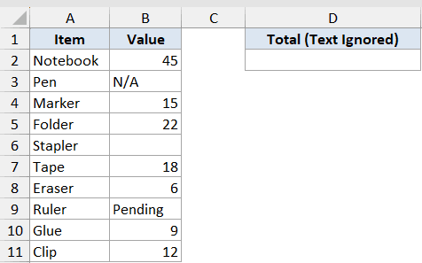
You want to total the Value column even though it has text and a blank mixed in.
Here is the formula:
=SUM(B2:B11)
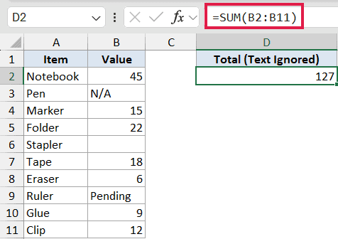
SUM quietly skips the “N/A”, “Pending”, and blank cells, so it still returns a total of 127.
Writing =B2+B3+B4… instead would return a #VALUE! error the moment it hits a text cell, so SUM saves you that headache.
Pro Tip: If a number looks right but SUM ignores it, it is probably stored as text (left-aligned, with a small green triangle). Convert it to a real number and it will be included.
Example 4: Add Up Only the Rows That Match
Sometimes you only want to total the rows that meet a condition. SUM can do that when you pair it with FILTER.
Here we have names in column A, regions in column B, and sales in column C, across twelve rows covering West, East, and South.
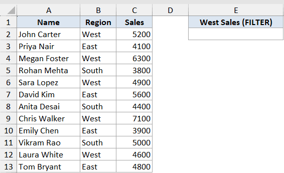
You want to add up only the sales from the West region using a dynamic array formula.
Here is the formula:
=SUM(FILTER(C2:C13,B2:B13="West"))
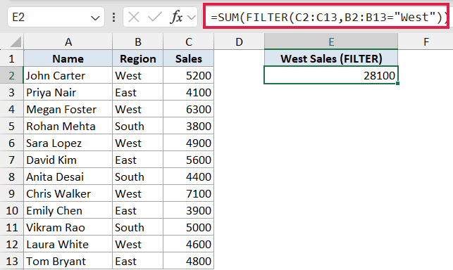
FILTER pulls out just the West rows as a list, and SUM adds them up to 28100.
You would get the same answer with =SUMIF(B2:B13,”West”,C2:C13), but FILTER also handles OR logic and more complex conditions. This approach needs Excel 365.
Example 5: Multiply and Add in One Step
There are times when SUM alone is not the leanest tool. Adding up a quantity times price is a classic case.
Here we have items in column A, quantity in column B, and price in column C, across seven rows.
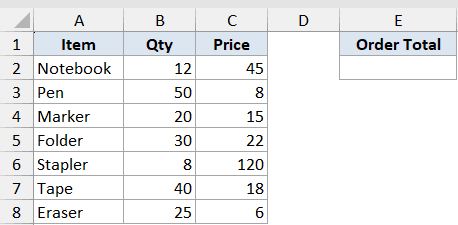
You want to work out the total order value, which is quantity times price for every row, all added up.
Here is the formula:
=SUMPRODUCT(B2:B8,C2:C8)
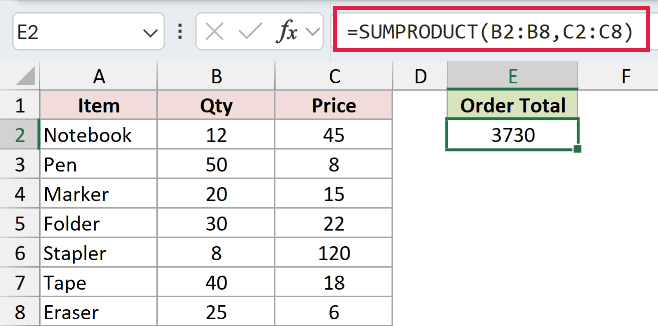
Plain SUM would need a helper column (=B2*C2) first, then a second step to total it.
SUMPRODUCT multiplies the two columns row by row and adds the results in one step, returning 3730.
Example 6: Sum the Same Cell Across Sheets
SUM can reach across worksheets, not just within one. This is handy for monthly tabs that all share the same layout.
Here we have three monthly tabs named Jan, Feb, and Mar, each with a Category column and a Sales column, with the month total sitting in cell B6. A separate Quarter Total tab pulls them together.
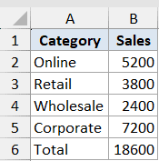
You want to add up the monthly totals in cell B6 from the Jan, Feb, and Mar sheets in a single formula.
Here is the formula:
=SUM(Jan:Mar!B6)
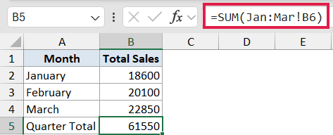
A 3D reference (SheetFirst:SheetLast!Cell) sums the same cell across every sheet from Jan through Mar, giving 61550.
The tabs must share the same layout, and if you insert another month’s tab between Jan and Mar, it gets included automatically.
One thing to know: SUMIFS and COUNTIFS cannot use 3D references, but SUM can. That makes SUM the go-to when you need a quick roll-up across identical sheets.
Tips and Common Mistakes
- Use AutoSum (Alt and =) to drop in a SUM formula in a second.
- SUM skips text and blanks, but it still passes through error values like #N/A, so fix the source error to clear it.
- To total only the visible rows of a filtered list, use SUBTOTAL or AGGREGATE instead of SUM.
- Numbers stored as text get skipped, so convert them to real numbers first.
- Use SUMIF or SUMIFS when you only want to add cells that meet a condition.
So that is the SUM function from end to end, from a simple column total to 3D references across sheets. Start with the basic range version, then reach for FILTER, SUMPRODUCT, or 3D references as your data gets trickier. Once these click, adding numbers in Excel stops being something you think about.
Related Excel Functions / Articles:
- SUMIF Function in Excel
- SUMIFS Function in Excel
- AVERAGE Function in Excel
- SUMPRODUCT vs SUMIFS Function in Excel
- AutoSum in Excel (Shortcut)
- Microsoft Excel Terminology (Glossary)
- How to Sum Positive Numbers in Excel (Formula)
- OFFSET Function in Excel
- List.Sum Function (Power Query M)
- SUMIFS with multiple sum columns
