If you want a quick way to check whether a cell holds a #N/A error, the ISNA function is what you need.
It returns TRUE when the value is the #N/A error and FALSE for anything else, including other error types like #VALUE!, #REF!, or a regular number or text value.
In Excel 365, you can also feed ISNA a range and the results spill into the cells below. In this article, I’ll show you how ISNA works with a few practical examples.
ISNA Function Syntax in Excel
Here is the syntax of the ISNA function:
=ISNA(value)
- value – The value you want to check. This can be a cell reference, a range, a formula result, or a literal value. ISNA returns TRUE if the value is the #N/A error, and FALSE for everything else.
One thing worth knowing right away. ISNA only catches the #N/A error. Other errors like #VALUE!, #REF!, #DIV/0!, and #NAME? all return FALSE. If you want to catch every error type, ISERROR is the broader cousin. If you specifically want to handle #N/A from a lookup formula, IFNA (Excel 2013 and later) is the modern shortcut.
When to Use ISNA Function
Use this function when you need to:
- Flag cells in a column where a lookup returned #N/A
- Find which items in one list are missing from another using ISNA with MATCH
- Replace #N/A errors from VLOOKUP with a friendly message
- Count how many lookups failed in a range
- Pull a clean list of missing items out of a comparison
Let me show you a few practical examples of how to use ISNA.
Example 1: Spot #N/A Errors in a Column
Let’s start with a simple example to see ISNA in its most basic form.
Below is the dataset. I have a column of VLOOKUP results in column A. Some lookups returned an email address, others came back as #N/A because the value wasn’t in the source table.
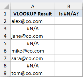
I want a TRUE or FALSE next to each row so I can see at a glance which lookups failed.
Here is the formula:
=ISNA(A2:A9)
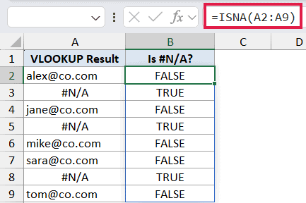
In the above formula, I’m feeding ISNA the entire range A2:A9 in one shot. Since ISNA spills in Excel 365, you only need to type the formula once in cell B2 and the results fill down to B9 automatically.
The three rows that came back as #N/A return TRUE. The five rows that returned an actual email return FALSE. Notice that ISNA only fires on #N/A. A regular number, text value, or any other error type would return FALSE.
Pro Tip: If you are on an older version of Excel that does not support dynamic arrays, type =ISNA(A2) in B2 and drag it down through B9. Same result, just the legacy way of doing it.
Example 2: Find Items Missing from Another List
Here’s where ISNA really earns its keep.
Pairing ISNA with MATCH is the standard way to compare two lists and flag the items that don’t show up in both. MATCH returns the position when it finds the item and #N/A when it doesn’t. ISNA turns that into a clean TRUE or FALSE.
Below is the dataset. I have a master inventory list in column A and a list of items that actually sold in column D. I want to flag the items that did not sell.
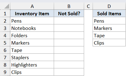
I want a TRUE or FALSE next to each inventory item, where TRUE means the item is missing from the sold list.
Here is the formula:
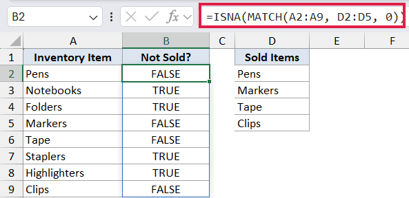
=ISNA(MATCH(A2:A9, D2:D5, 0))
How this formula works:
- MATCH looks up each value in A2:A9 against the sold list in D2:D5. When it finds a match, it returns the position as a number. When it doesn’t, it returns #N/A.
- ISNA wraps that result. #N/A means the item is missing from the sold list, so ISNA returns TRUE. A number means the item sold, so ISNA returns FALSE.
Pens, Markers, Tape, and Clips return FALSE since they appear in the sold list. Notebooks, Folders, Staplers, and Highlighters return TRUE, which tells us those four items are sitting in inventory unsold.
Pro Tip: The third argument in MATCH is set to 0, which forces an exact match. Leave that out and MATCH switches to approximate match mode, which gives you wrong results on an unsorted list.
Example 3: Show a Friendly Message Instead of #N/A in VLOOKUP
Here’s the classic ISNA pattern most people learn first.
When a VLOOKUP can’t find what it’s searching for, it returns #N/A. That’s fine for you, but on a shared report it looks broken. Wrapping the VLOOKUP in IF and ISNA lets you swap that error for a friendly message instead.
Below is the dataset. I have an employee lookup table in columns A and B with names and email addresses. In column D, I have a list of names I want to look up.
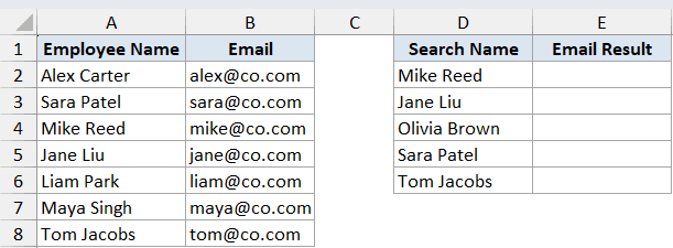
I want the email address next to each search name, but a clean “Not Found” instead of #N/A when the name isn’t in the table.
Here is the formula:
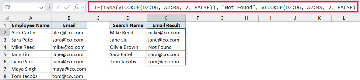
=IF(ISNA(VLOOKUP(D2:D6, A2:B8, 2, FALSE)), "Not Found", VLOOKUP(D2:D6, A2:B8, 2, FALSE))
How this formula works:
- VLOOKUP looks up each name in D2:D6 against the table A2:B8 and tries to return the email from column 2. For names in the table it returns the email. For Olivia Brown, who isn’t in the table, it returns #N/A.
- ISNA wraps that result. If VLOOKUP returned #N/A, ISNA gives TRUE. Otherwise FALSE.
- IF then picks the right output. TRUE means use “Not Found”, FALSE means run VLOOKUP a second time to fetch the actual email.
You get the email address for Mike Reed, Jane Liu, Sara Patel, and Tom Jacobs, and “Not Found” for Olivia Brown.
> In Excel 2013 and later, you can also do this with IFNA: =IFNA(VLOOKUP(D2:D6, A2:B8, 2, FALSE), "Not Found"). That’s a lot shorter because you don’t have to type the VLOOKUP twice. The ISNA version still works (and is the only option in older Excel versions where IFNA doesn’t exist), so it’s worth knowing both. Excel 365 users can take it one step further with XLOOKUP: =XLOOKUP(D2:D6, A2:A8, B2:B8, "Not Found"), which has the not-found message built right into its arguments.
Example 4: Count How Many Lookups Failed
Let’s wrap up with a quick count.
Sometimes you don’t need to label every row, you just want to know how many lookups in a column came back as #N/A. ISNA inside SUMPRODUCT gives you that in one cell.
Below is the dataset. I have a column of VLOOKUP results in column A. Some are actual email addresses, others are #N/A.
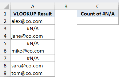
I want a single number in cell C2 that tells me how many lookups in column A came back as #N/A.
Here is the formula:
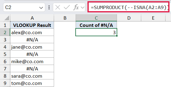
=SUMPRODUCT(--ISNA(A2:A9))
How this formula works:
- ISNA(A2:A9) returns an array of TRUE and FALSE values, one per row.
- The double minus (–) coerces those into 1s and 0s. TRUE becomes 1, FALSE becomes 0.
- SUMPRODUCT adds them up, giving you the count of #N/A errors.
In this example, the result is 3 since the column has three #N/A entries and five working email addresses.
Pro Tip: COUNTIF can do this in one shot too: =COUNTIF(A2:A9, NA()). That said, the SUMPRODUCT + ISNA pattern is useful when you want to combine the #N/A test with other conditions, or when you’re on a pre-365 Excel where SUM applied to an array needs Ctrl+Shift+Enter to work. SUMPRODUCT handles the array entry on its own.
Example 5: Extract the List of Missing Items
Let’s step it up with a more useful scenario.
Sometimes you don’t just want a TRUE/FALSE flag for missing items, you want a clean list of which ones are missing. FILTER with ISNA and MATCH does that in a single formula.
Below is the dataset. I have a list of invited guests in column A and a list of guests who actually attended in column C. I want a third column that pulls out just the names of the guests who didn’t show up.
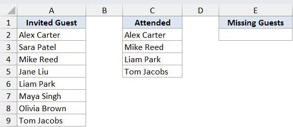
I want a clean list in column E that contains only the names from column A that don’t appear in column C.
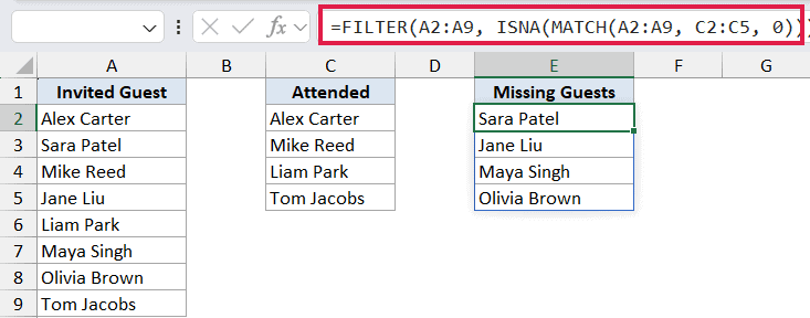
Here is the formula:
=FILTER(A2:A9, ISNA(MATCH(A2:A9, C2:C5, 0)))
How this formula works:
- MATCH compares each invited guest in A2:A9 against the attendee list in C2:C5. It returns a position number for guests who attended and #N/A for guests who didn’t.
- ISNA turns that result into a TRUE/FALSE array. TRUE means the guest is missing from the attended list.
- FILTER takes that TRUE/FALSE array as its include test. It keeps only the rows where the test returns TRUE.
- The result spills into column E, showing only the guests who didn’t show up.
You get Sara Patel, Jane Liu, Maya Singh, and Olivia Brown in column E, which are the four invited guests who didn’t make it to the event.
Tips & Common Mistakes
- ISNA only catches the #N/A error. Other errors like #VALUE!, #REF!, #DIV/0!, #NUM!, #NAME?, and #NULL! all return FALSE. If you want to catch every error type at once, use ISERROR instead.
- #N/A and the text string “N/A” are different things. A cell containing the literal text “N/A” (typed by hand) returns FALSE in ISNA, because it’s just text, not an error. Only the actual #N/A error value triggers TRUE.
- IFNA is a cleaner alternative for lookup formulas. In Excel 2013 and later,
=IFNA(VLOOKUP(...), "Not Found")does the same job as=IF(ISNA(VLOOKUP(...)), "Not Found", VLOOKUP(...))without typing the lookup twice. - IFERROR catches too much. It looks tempting to swap IF/ISNA with IFERROR, but IFERROR also hides genuine problems like #VALUE! or #REF!. Use IFNA when you only want to catch the “not found” case.
- Pair it with MATCH for list comparisons. The
ISNA(MATCH(...))pattern is the most common way to check whether a value exists in another list. Combine it with FILTER to pull out the missing items, or with SUMPRODUCT to count them. - Pair it with ISTEXT or ISNUMBER for non-error checks. ISNA is the right tool when you specifically care about #N/A. If you need to know whether a cell is text, a number, or blank, the other IS-family functions are the cleaner choice.
- Watch the third argument of MATCH. Always pass 0 (exact match) when you’re using MATCH inside ISNA for list comparisons. The default approximate match silently returns wrong positions on unsorted data, which makes ISNA return FALSE when it should be TRUE.
That covers the main ways ISNA shows up in real spreadsheets. On its own it’s a one-line check for the #N/A error. But pair it with MATCH to compare lists, with VLOOKUP and IF to clean up lookup output, or with FILTER to extract the missing items, and it quietly does a lot of work.
Related Excel Functions / Articles:
- MATCH Function in Excel
- VLOOKUP Not Working – 7 Possible Reasons + Fix!
- Check If Value is in List in Excel
- XLOOKUP Vs INDEX MATCH in Excel
- #REF! Error in Excel
- #DIV/0! Error in Excel – How to Fix It?
- How to Compare Two Cells in Excel? (Exact/Partial Match)
- Bulk Find and Replace in Excel
- ISBLANK Function in Excel
- IFERROR Function in Excel