If you want to catch errors in your formulas and show something useful instead, like a friendly message, a zero, or a blank cell, the IFERROR function is what you’re looking for.
It checks a formula for any error and lets you decide what to display when one shows up.
In Excel 365, you can also feed IFERROR a range and the results will spill into the cells below.
IFERROR Function Syntax in Excel
The IFERROR function checks a value for an error and returns a result you specify if it finds one.
=IFERROR(value, value_if_error)
- value: the formula or cell you want to check for an error.
- value_if_error: what to return if the first argument evaluates to an error. This can be a number, text in quotes, a blank (“”), or even another formula.
IFERROR catches all the common error types: #N/A, #VALUE!, #REF!, #DIV/0!, #NUM!, #NAME?, and #NULL!. If the value doesn’t return an error, IFERROR simply gives you the original result.
When to Use IFERROR Function
Here are some everyday situations where IFERROR comes in handy:
- Hiding division errors when a denominator is zero or blank.
- Showing a clear “not found” message when a VLOOKUP or lookup fails.
- Returning a blank cell so error codes don’t clutter a report.
- Adding up a column that has a few stray errors in it.
- Building a fallback that checks a second table when the first one comes up empty.
Example 1: Replace #DIV/0! Errors With a Message
Let’s start with the most common reason people reach for IFERROR.
Below is a dataset with each store’s total sales and the number of orders they took. We want the average sale per order, which means dividing sales by orders.
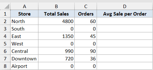
The problem is that a few stores had no orders at all, so dividing by zero gives a #DIV/0! error. We want those rows to say “No Orders” instead.
Here is the formula:
=IFERROR(B2:B8/C2:C8,"No Orders")
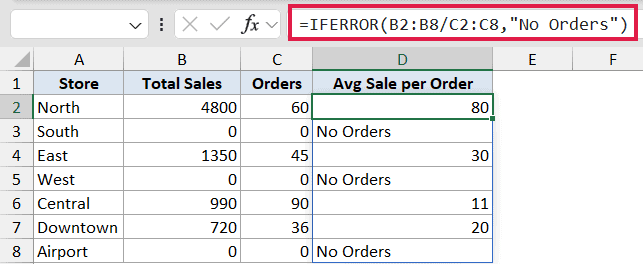
The division B2:B8/C2:C8 runs down the whole column at once. Wherever orders are zero, the division would normally fail, so IFERROR swaps that error for the text “No Orders”. Every other row shows the actual average.
Since this is entered once in the top cell and feeds whole ranges, the results spill down automatically in Excel 365. In older versions you’d put =IFERROR(B2/C2,"No Orders") in the first cell and copy it down.
Example 2: Wrap VLOOKUP for a Friendly Not Found Message
Here’s another scenario that comes up all the time.
Below is a small price list on the left, and a few items we want to look up on the right. We’re using VLOOKUP to pull each item’s price from the list.
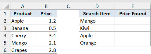
Some of the search items aren’t in the price list at all, and a plain VLOOKUP would return the #N/A error for those. We want it to say “Not in list” instead.
Here is the formula:
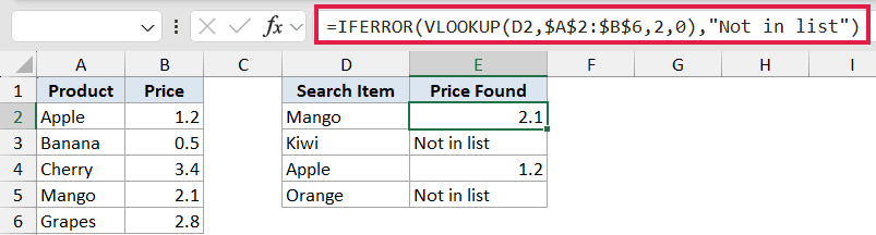
=IFERROR(VLOOKUP(D2,$A$2:$B$6,2,0),"Not in list")
How this formula works:
- VLOOKUP looks for the item in D2 inside the price list in A2:B6 and returns its price.
- If the item isn’t found, VLOOKUP returns #N/A.
- IFERROR catches that #N/A and shows “Not in list” instead.
This is probably the single most popular use of IFERROR, because a raw #N/A in a report looks broken to anyone reading it.
In Excel 365, you can also do this with XLOOKUP, which has a built-in spot for the not-found result: =XLOOKUP(D2,$A$2:$A$6,$B$2:$B$6,"Not in list"). That’s a bit cleaner since you don’t need to wrap anything. The IFERROR plus VLOOKUP version still works everywhere though, including older versions where XLOOKUP isn’t available, so it’s worth knowing both.
Example 3: Return a Blank Cell Instead of an Error
Sometimes you don’t want any message at all. You just want the cell to look empty.
Below is an order sheet with a quantity and a unit price for each item. We want to calculate the total by multiplying the two.
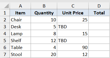
A couple of rows have “TBD” typed in the unit price because the price hasn’t been set yet. Multiplying a number by text gives a #VALUE! error, so we want those rows to stay blank until the price is filled in.
Here is the formula:
=IFERROR(B2:B7*C2:C7,"")
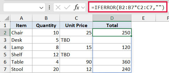
The two empty quotes (“”) tell IFERROR to return nothing when it hits an error. So the rows with “TBD” come back blank, while the rows with real prices show their totals. This also shows that IFERROR isn’t just for division errors, it catches the #VALUE! error here too.
A quick word of caution. A cell that looks blank because of IFERROR isn’t truly empty, it holds an empty text string. So if you later run a formula like COUNTBLANK over the column, it won’t count those cells as blank.
Example 4: Sum a Range That Contains Errors
Here’s a handy trick for when errors get in the way of a simple total.
Below is a list of stores with their revenue and how many days each was open. We want to add up the daily averages, which is revenue divided by days for each store.
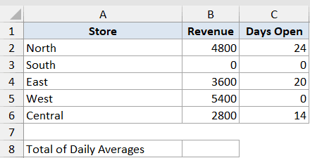
Two of the stores were open zero days, so their daily average would be a #DIV/0! error. A normal SUM would choke on those errors and return an error itself. We want it to just skip them and add the rest.
Here is the formula:
=SUM(IFERROR(B2:B6/C2:C6,0))
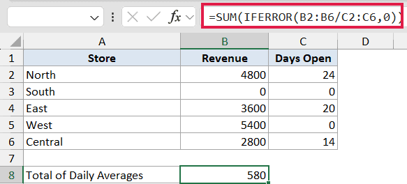
Working from the inside out, IFERROR turns each store’s daily average into a number, replacing any #DIV/0! error with a 0. SUM then adds up that clean list of numbers, so the error rows simply contribute nothing to the total.
This pattern of wrapping a calculation in IFERROR before passing it to SUM (or AVERAGE, or COUNT) is a clean way to keep a few bad rows from breaking your whole total.
Example 5: Nested IFERROR for a Fallback Lookup
Let’s step it up with a more complex use case.
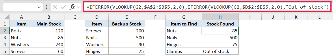
Below are two stock lists, a main warehouse on the left and a backup warehouse in the middle. On the right are the items we need to find. We want to check the main warehouse first, and if the item isn’t there, check the backup.
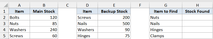
If the item isn’t in either warehouse, we want to show “Out of stock”. This is where you can nest one IFERROR inside another.
Here is the formula:
=IFERROR(VLOOKUP(G2,$A$2:$B$5,2,0),IFERROR(VLOOKUP(G2,$D$2:$E$5,2,0),"Out of stock"))
How this formula works:
- The first VLOOKUP searches the main warehouse (A2:B5). If it finds the item, you get its stock and you’re done.
- If the main warehouse comes up empty, the first IFERROR runs its second argument, which is another VLOOKUP against the backup warehouse (D2:E5).
- If the backup warehouse also comes up empty, the inner IFERROR returns “Out of stock”.
You can keep nesting IFERROR like this for a third or fourth fallback, though once you get past two or three levels it’s usually cleaner to rethink the layout or use a single combined lookup table.
Tips & Common Mistakes
- IFERROR hides every error, even the ones you didn’t expect. If your formula has a typo that throws a #NAME? error, IFERROR will quietly mask it along with the errors you meant to catch. Build and test your formula first, then wrap it in IFERROR once you know it works.
- Catch only not-found errors when that’s all you want. If you specifically want to handle #N/A from a lookup but still see other errors like #DIV/0!, the IFNA function catches only #N/A and leaves the rest visible. You can get the same targeted behavior by wrapping your lookup with the ISNA function inside an IF, which can save you from accidentally hiding a real problem.
- A blank from IFERROR isn’t truly empty. Returning “” gives you an empty text string, not an empty cell. Formulas like ISBLANK and COUNTBLANK won’t treat it as blank, so keep that in mind if you reference the column later.
- IFERROR needs at least Excel 2007. In older versions you’d combine IF with ISERROR, like
=IF(ISERROR(formula),value_if_error,formula), which repeats the formula twice. IFERROR does the same job in one shot.
IFERROR is a small function that keeps ugly error codes out of your spreadsheets. The trick is deciding what should show up in place of the error, whether that’s a clear message, a zero, or a blank cell. Once you get used to it, you’ll find yourself wrapping it around almost any formula that might trip up.
Related Excel Functions / Articles: