
The MIRR function in Excel returns a modified internal rate of return for cash flows occurring at regular intervals.
You specify separate rates for financing negative cash flows and reinvesting positive cash flows. This makes those assumptions explicit when comparing investment returns.
The result is a rate per cash-flow period, so the interval between entries matters when interpreting it.
In this article, I’ll show you how to calculate a modified return, test financing and reinvestment rates, and compare MIRR with IRR.
MIRR Function Syntax in Excel
The MIRR function needs a cash-flow series and two rates for the same period used by those cash flows.
=MIRR(values,finance_rate,reinvest_rate)
valuesis the required cash-flow range. It must contain at least one negative payment and one positive receipt.finance_rateis the required interest rate paid on money used to finance the cash flows.reinvest_rateis the required rate earned when positive cash flows are reinvested.
MIRR reads the cash flows in their worksheet order. Enter payments as negative values, receipts as positive values, and keep the periods evenly spaced.
When to Use MIRR Function
- Calculate a periodic investment return with separate finance and reinvestment assumptions.
- Compare projects using more realistic reinvestment rates than a standard IRR calculation.
- Test how changes in either rate affect the return.
- Calculate the return for one project selected from a larger cash-flow table.
Example 1: Calculate Annual MIRR
Let’s begin with a standard annual cash-flow series.
Below is the maintenance-retrofit cash flow with annual finance and reinvestment rates, plus an empty result cell.
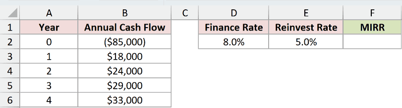
I want to calculate the retrofit’s annual modified internal rate of return.
Here is the formula:
=MIRR(B2:B6,D2,E2)
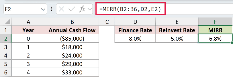
The formula returns 6.8%. The cash flows are annual, so the 8% finance rate, 5% reinvestment rate, and MIRR result are all annual rates.
MIRR uses the negative initial cost in B2 as a payment. The positive values in B3:B6 are the later cash receipts.
Pro Tip: Match both rate inputs to the cash-flow period. Monthly cash flows need monthly rates, while annual cash flows need annual rates.
Example 2: MIRR Finance Rate Sensitivity
This example tests the cost of financing.
Below is a facility-upgrade cash flow with three finance rates, a fixed reinvestment rate in G2, and empty MIRR cells.
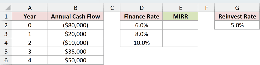
I want to see how MIRR changes as the finance rate moves from 6% to 10%.
Enter this formula in E2 and copy it down through E4:
=MIRR($B$2:$B$6,D2,$G$2)
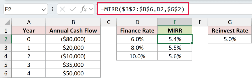
The formula returns 5.4%, 5.5%, and 5.6% for finance rates of 6%, 8%, and 10%.
The cash-flow range and reinvestment rate stay fixed. D2 changes by row so each copied formula uses the finance rate beside it.
The Year 2 cash shortfall makes the finance rate matter because MIRR discounts that later payment.
If the initial outlay were the only negative cash flow, changing the finance rate would not affect this example’s result.
Example 3: MIRR Reinvestment Rate Sensitivity
Now let’s vary the rate earned on positive cash flows.
Below is an equipment-lease cash flow with three reinvestment rates, a fixed finance rate in G2, and empty MIRR cells.
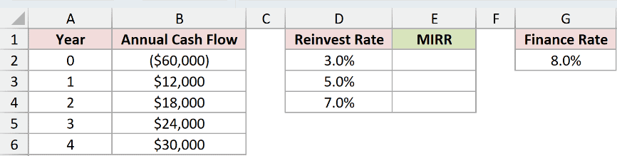
I want to see how the return changes as the reinvestment rate rises from 3% to 7%.
Enter this formula in E2 and copy it down through E4:
=MIRR($B$2:$B$6,$G$2,D2)
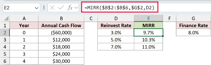
The results are 9.7%, 10.3%, and 11.0% for reinvestment rates of 3%, 5%, and 7%.
The finance rate stays fixed at 8% in G2. D2 changes by row, so the copied formulas test each reinvestment rate against the same cash flows.
Pro Tip: A higher assumed reinvestment rate can raise MIRR. Use a rate you can reasonably expect to earn instead of choosing one to improve the result.
Example 4: Compare MIRR With IRR
Here’s a direct comparison using one cash-flow series.
Below is the service-center expansion cash flow with empty cells for IRR and MIRR.
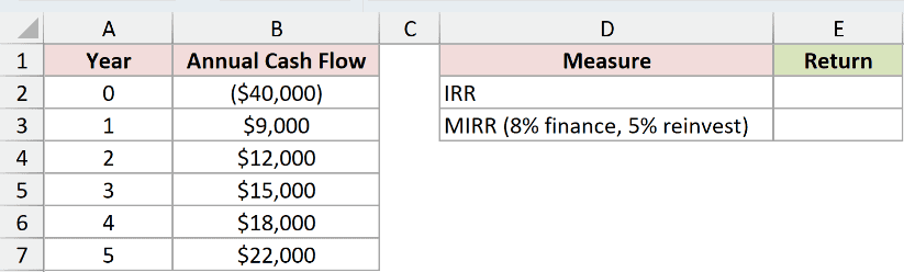
I want to compare the standard internal rate of return with MIRR using 8% finance and 5% reinvestment rates.
First, here is the IRR formula:
=IRR(B2:B7)
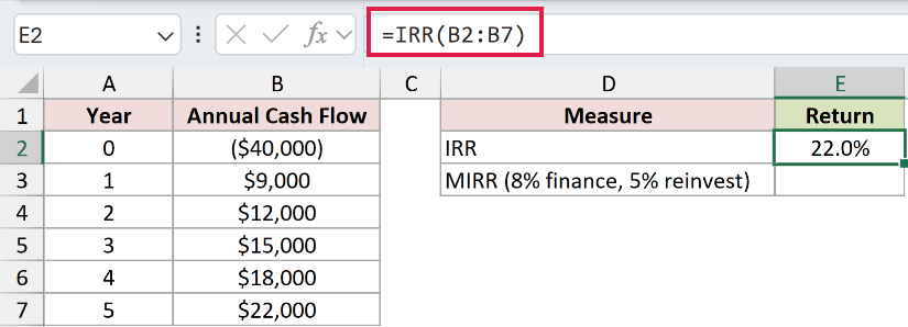
IRR returns 22.0%. It finds the rate at which this cash-flow series has a net present value of zero.
Now calculate MIRR with the two stated rate assumptions:
=MIRR(B2:B7,0.08,0.05)
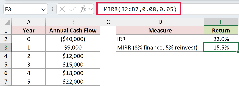
MIRR returns 15.5%. The results differ because MIRR uses the 8% finance rate and 5% reinvestment rate supplied in the formula.
Use IRR when its single-return framework suits the analysis. Use MIRR when you want the financing and reinvestment assumptions stated separately.
Example 5: MIRR for Filtered Cash Flows
Let’s calculate the return for one project selected from a combined table.
Below are alternating Atlas and Beacon cash flows in chronological order, with controls for the selected project and both annual rates.
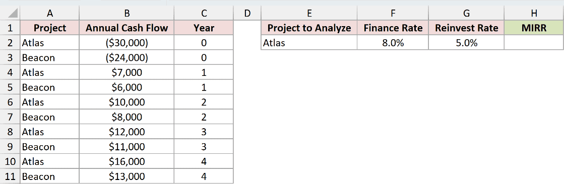
I want to calculate MIRR for the Atlas rows selected in cell E2.
Here is the formula:
=MIRR(FILTER(B2:B11,A2:A11=E2),F2,G2)
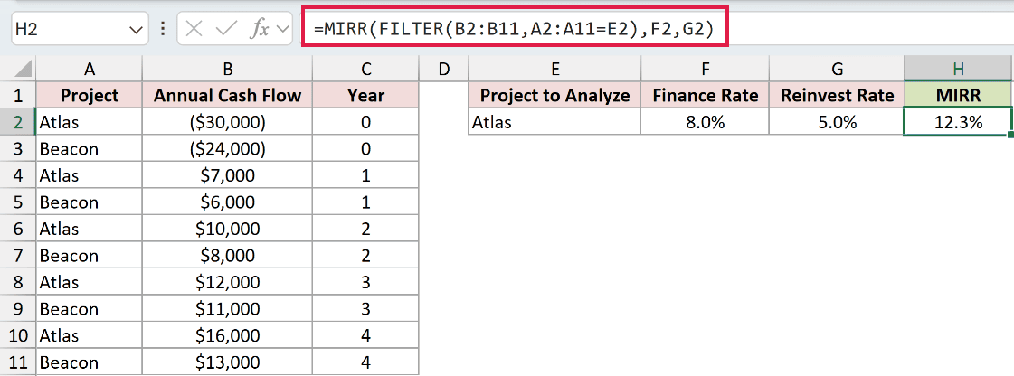
FILTER returns the Atlas cash flows while preserving their worksheet order. MIRR then applies the 8% finance rate and 5% reinvestment rate.
The result is 12.3%. Change E2 to Beacon, and the same formula recalculates the selected project’s annual return.
FILTER is available in Excel 2021 and later. In Excel 2019 or earlier, place each project’s cash flows in a separate helper range before using MIRR.
Pro Tip: Keep the filtered rows in chronological order and include the initial negative cash flow. MIRR needs at least one negative and one positive value.
Tips & Common Mistakes
- Keep the cash flows at regular intervals. Use XIRR when actual transaction dates are uneven.
- Enter payments as negative values and receipts as positive values.
- Include at least one negative and one positive cash flow, or MIRR returns
#DIV/0!. - Keep zero-value periods as zeros when they represent real periods. MIRR includes zero but ignores text, logical values, and empty cells in referenced ranges.
- Match the finance rate and reinvestment rate to the cash-flow period.
I covered a basic MIRR calculation, both rate assumptions, an IRR comparison, and a selected project built with FILTER.
I hope you found this article helpful.
