If you want to know what return a series of cash flows is actually earning you, like an investment that costs money up front and pays you back over several years, the IRR function works it out in one step.
IRR stands for internal rate of return. It’s the single interest rate at which all your cash flows, the money out and the money in, balance out to zero.
IRR returns a single rate, but it works happily inside dynamic array formulas like =IRR(FILTER(…)). I’ll show you that along with four other examples below.
IRR Function Syntax in Excel
Here is the syntax of the IRR function:
=IRR(values,[guess])
- values: A range of cells with your cash flows. It needs at least one negative number (cash out) and one positive number (cash in), in date order.
- [guess]: Optional. Your rough estimate of the rate. If you leave it out, Excel starts at 10%.
When to Use IRR Function
- When you want the return rate on an investment that pays back over regular periods, like years or months.
- When you’re comparing two projects and want to see which one earns more.
- When you need a single number to judge whether a project clears your target return.
- When your cash flows happen at even intervals (use XIRR instead if the dates are irregular).
Example 1: IRR of a Project’s Cash Flows
Let’s start with a straightforward project.
Below is the dataset. Column A lists the years and column B lists the cash flow for each year. Year 0 is the initial investment, shown as a negative number, followed by five years of returns.
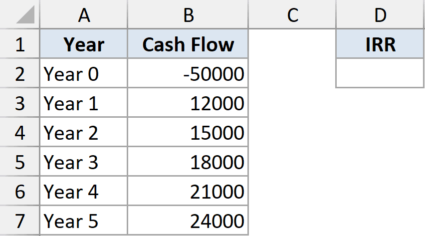
I want the internal rate of return across the whole series in B2:B7.
Here is the formula:
=IRR(B2:B7)
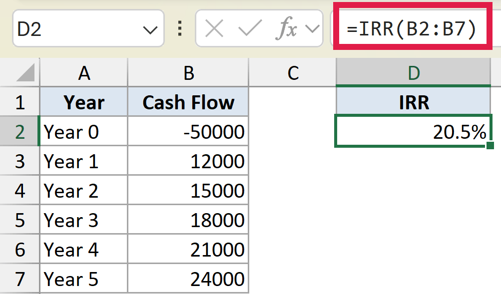
IRR looks at the 50,000 paid out and the growing returns that follow, then finds the rate that makes them balance. That works out to about 20.5%.
In plain terms, this project earns the equivalent of a 20.5% annual return. The first value has to be negative, since you can’t have a return without first putting money in.
Pro Tip: IRR returns a decimal, so format the cell as a percentage to read it as 20.5% instead of 0.205. Select the cell and press Ctrl + Shift + %.
Example 2: Compare Two Investment Options
IRR really earns its keep when you’re choosing between options.
Below is the dataset. Column A lists the years, and columns B and C hold the cash flows for two small businesses you could invest in: a cafe and a food truck.
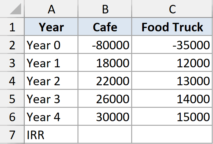
I want the IRR for each option so I can compare them side by side.
Here is the formula for the cafe:
=IRR(B2:B6)
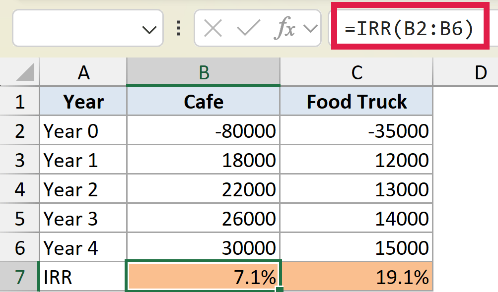
And here is the formula for the food truck:
=IRR(C2:C6)
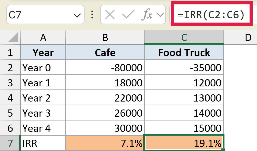
The cafe needs a bigger investment up front and returns about 7.1%. The food truck costs far less and returns about 19.1%.
Even though the cafe brings in more total cash, the food truck earns a much higher rate on the money you put in. That’s the kind of insight IRR is built for.
Example 3: Monthly IRR and Annualizing It
When your cash flows are monthly, IRR gives you a monthly rate. You usually want to turn that into an annual figure.
Below is the dataset. Column A lists the months and column B lists the monthly cash flow, starting with the amount paid out in month 0.
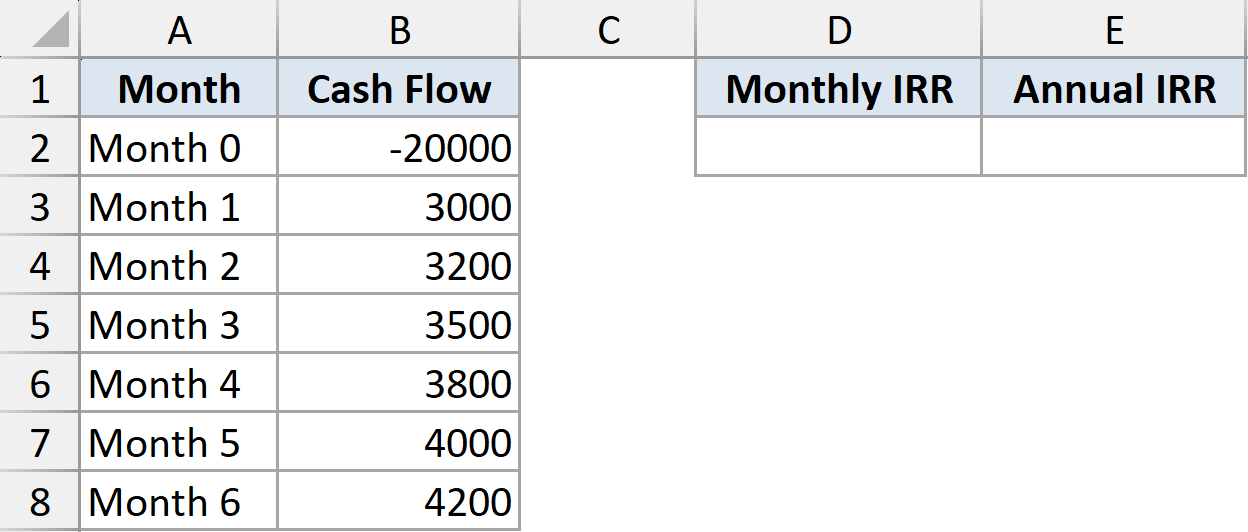
I want the monthly IRR first, then the annual rate that it works out to.
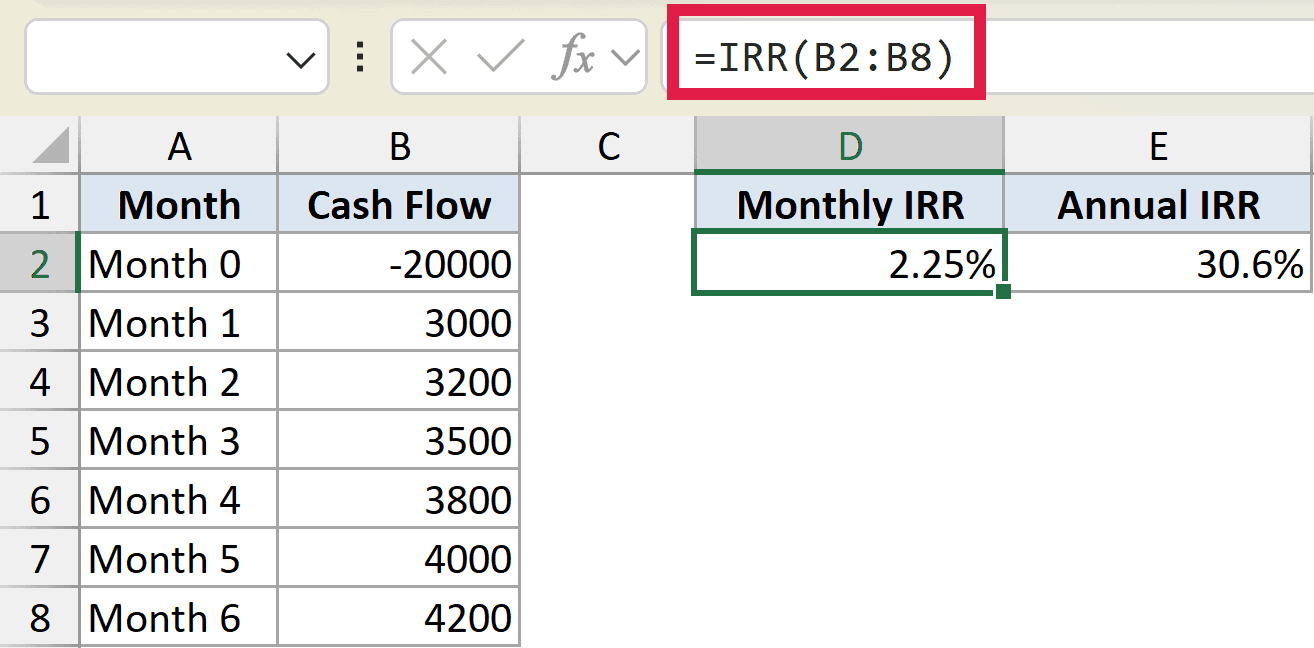
Here is the formula for the monthly IRR:
=IRR(B2:B8)
And here is the formula to annualize it:
=(1+D2)^12-1
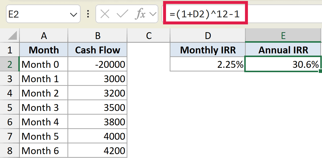
The first formula gives a monthly IRR of about 2.25%. The second compounds that across 12 months to get the true annual rate, about 30.6%.
Compounding is the right way to do this. Simply multiplying the monthly rate by 12 would overstate the return.
Example 4: IRR with a Mid-Project Investment
Real projects aren’t always one payment out followed by steady returns. Sometimes you put more money in partway through.
Below is the dataset. Column A lists the years and column B lists the cash flows, including an extra investment in Year 3 shown as a negative number.
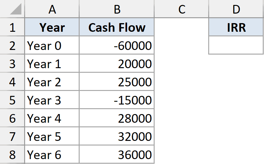
I want the IRR across the full series, even with that mid-project outflow.
Here is the formula:
=IRR(B2:B8)
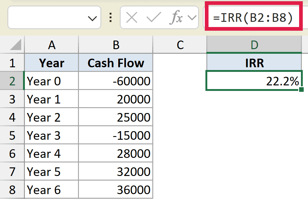
IRR handles the mix of negatives and positives without any trouble, returning about 22.2%.
As long as the cash flows are in date order, IRR reads them just as they happen. The Year 3 top-up is simply treated as money going out in that period.
Example 5: IRR on a Dynamic Subset with FILTER
IRR doesn’t spill on its own, but you can feed it a dynamic array. Here we use FILTER to compute IRR through a chosen number of years.
Below is the dataset. Column A lists the year numbers, column B lists the cash flows, and cell D2 holds how many years to include.
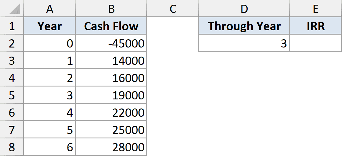
I want the IRR using only the cash flows up to the year number in D2, which is 3.
Here is the formula:
=IRR(FILTER(B2:B8,A2:A8<=D2))
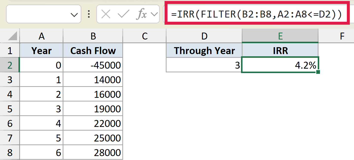
FILTER pulls the cash flows for years 0 through 3, and IRR finds the return across just that stretch, about 4.2%.
Raise D2 to include more years and the rate climbs as the later returns come in. It’s a quick way to see how the return builds over the life of a project.
Tips & Common Mistakes
- A #NUM! error usually means there’s no sign change in your data. IRR needs at least one negative and one positive value to solve.
- If you still get #NUM!, supply a guess close to your expected rate, like 0.05 or 0.5, to help Excel land on the right answer.
- The order of the values matters. IRR treats them as one cash flow per period, so keep them in date order.
- IRR ignores blank cells, text, and TRUE/FALSE values. If a period truly has no cash flow, enter a 0 so the timing stays correct.
- IRR is closely tied to net present value. It’s simply the discount rate at which a project’s NPV comes out to zero.
- When the gaps between cash flows are uneven, use XIRR instead. It takes actual dates and gives you an annual rate directly.
IRR turns a column of cash flows into a single number you can act on, which makes it one of the most useful functions for any kind of financial decision.
Work through the examples above and you’ll be comparing investments with confidence. For a step-by-step walkthrough, see our guide on how to calculate IRR in Excel.
Related Excel Functions / Articles: