If you want the annual return on an investment whose cashflows happen on irregular dates, XIRR is the function you reach for.
Plain IRR assumes every cashflow is one equal period apart, so it gets the number wrong the moment your dates are uneven.
This article walks through the syntax and four real examples so you can pull a clean annualized return from any dated cashflow series. XIRR returns a single rate, so it does not spill, and each formula gives you one annualized return.
XIRR Function Syntax in Excel
Here is how the XIRR function is built:
=XIRR(values, dates, [guess])
- values (required) – the series of cashflows. Money you put in is negative, money you get back is positive. You need at least one of each.
- dates (required) – the date for each cashflow, one per value, same count as values.
- guess (optional) – a starting estimate for the rate. Defaults to 0.1 (10%); only matters when the default fails to find an answer.
XIRR returns the single annual rate of return that accounts for exactly when each cashflow happened.
When to Use XIRR Function
- Finding the return on an account where you add and withdraw money on irregular dates.
- Measuring private equity or real estate cashflows that land on arbitrary dates.
- Working out the return on a SIP or recurring investment that ends in a redemption value.
- Comparing dated deals on one annual figure so you can line them up side by side.
Example 1: Annual return on dated cashflows
Let’s start with the most common case, a lump sum you invest once and then get back in pieces over time.
Below is the dataset. Column A has the date of each cashflow and column B has the cashflow itself. The first row is the money invested, and the four rows below it are returns landing on uneven dates.
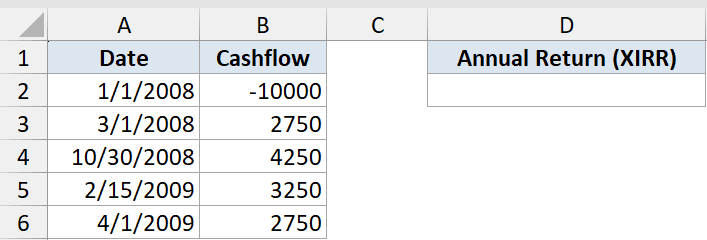
We want the annualized return on this investment where the returns arrive on uneven dates.
Here is the formula:
=XIRR(B2:B6,A2:A6)
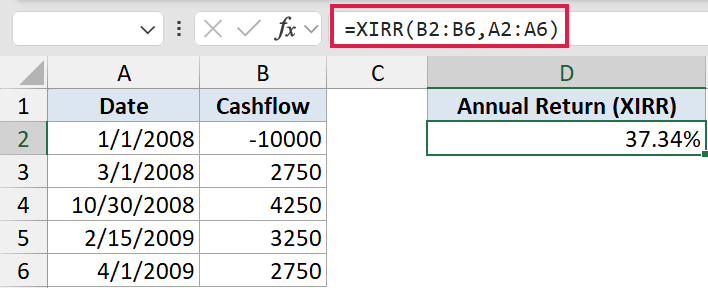
The first cashflow is the money invested, which is negative. The four later cashflows are returns, and each one sits on its own date.
XIRR finds the single annual rate that ties them all together. Here that rate works out to 37.34%.
Pro Tip: XIRR returns a raw decimal like 0.3734. Format the cell as Percentage to read it as 37.34%.
Example 2: XIRR vs IRR (why dates matter)
Now let’s see why the dates actually matter, by running XIRR and plain IRR on the exact same numbers.
Below is the dataset. Column A has the dates and column B has the cashflows. To the right, column D lists the method and column E holds each result.
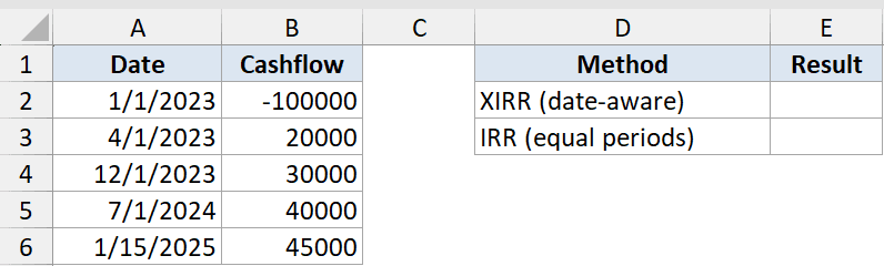
We want to compare XIRR against plain IRR on the exact same cashflows.
Here is the formula:
=XIRR(B2:B6,A2:A6)
That returns 25.55%. For comparison, here is the IRR version:
=IRR(B2:B6)
That returns 11.52%.
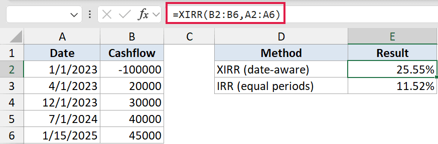
Here is why the two numbers split so far apart:
- XIRR reads the actual dates, so it knows the gaps between cashflows are uneven.
- IRR ignores the date column entirely and assumes every cashflow is one equal period apart.
- That mismatch is why the two numbers diverge so much, 25.55% versus 11.52%.
- Use XIRR whenever the timing is irregular, which is almost always for real investments.
Example 3: Fix a #NUM! error with the guess argument
Sometimes XIRR throws a #NUM! error even though your data looks fine. This usually means the default starting guess is too far from the real answer.
Below is the dataset. Column A has the dates and column B has the cashflows. This is a deal that lost almost everything, with only small amounts trickling back against a big upfront investment.
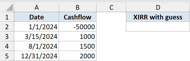
We want XIRR on a deal that lost almost everything, where the default cannot find an answer on its own.
Here is the formula:
=XIRR(B2:B5,A2:A5,-0.5)
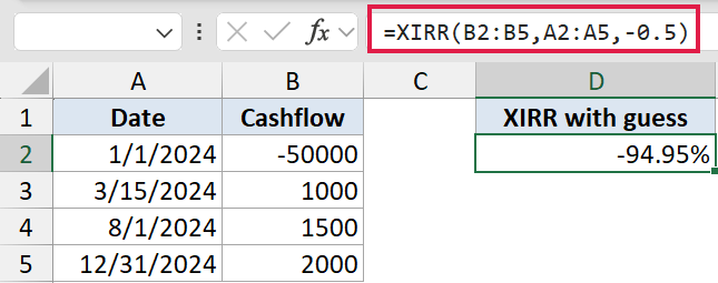
Only 4,500 comes back against a 50,000 investment, so the true rate is steeply negative.
XIRR starts from a 10% guess by default and may return #NUM! because it cannot reach the answer from there. Adding a third argument, the guess -0.5 (negative 50%), gives it a sensible starting point and it converges to about -94.95%.
Pro Tip: If XIRR returns #NUM! and you already have one negative and one positive cashflow, add a guess between -0.9 and 0.9. A negative result like this is not an error, it just means the investment lost money on an annualized basis.
Example 4: Annualized return on a SIP
Here is a case a lot of people care about, a SIP where you put in a fixed amount each month and then cash out at the end.
Below is the dataset. Column A has the date of each contribution and column B has the amount. The six monthly contributions are money out, and the final row is the redemption value.
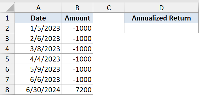
We want the annualized return on six monthly contributions that grew to a final value.
Here is the formula:
=XIRR(B2:B8,A2:A8)
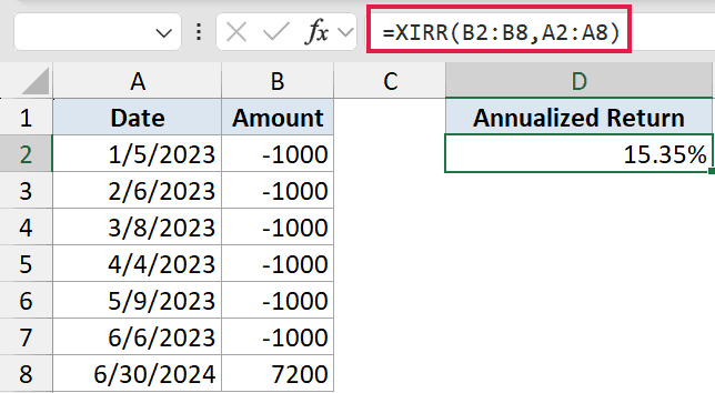
Each of the six contributions is negative money out on its own date, and the 7,200 final value is the money back. The result comes out to about 15.35%.
The contribution dates are not perfectly spaced, which is exactly why XIRR is the right tool. It weights each dollar by how long it stayed invested instead of averaging the monthly returns.
Tips & Common Mistakes
- You need at least one negative and one positive cashflow, or XIRR returns #NUM!. Money out is negative, money in is positive.
- Dates must be real Excel dates, not text. Text dates cause #VALUE! (check that they are right-aligned in the cell).
- values and dates must have the same count. A mismatch returns #NUM!.
- If XIRR cannot converge it returns #NUM!. Add a guess (a third argument) to fix it.
- The result is an annualized decimal, so format the cell as Percentage. XNPV is the sibling function: XIRR is exactly the rate at which XNPV equals zero.
XIRR is the function to use any time your cashflows land on dates that are not evenly spaced. Feed it the values and the matching dates, and it hands back one clean annual return.
If you ever hit a #NUM! error, reach for the guess argument before assuming your data is broken. Nine times out of ten that fixes it.
Related Excel Functions / Articles: