
The NOT function in Excel reverses a logical value: TRUE becomes FALSE, and FALSE becomes TRUE.
It is useful when a rule is easier to express by excluding a condition, such as checking that a value is not blank or an item is not approved.
In this article, I’ll show you how to reverse logical tests, identify nonblank cells, and filter out unwanted statuses.
NOT Function Syntax in Excel
The NOT function has one required argument:
=NOT(logical)
logicalis a value or expression that evaluates to TRUE or FALSE. NOT returns the opposite logical value.
When to Use the NOT Function
- Reverse a column of existing TRUE and FALSE values.
- Test whether text does not match a specified value.
- Make an IF formula act when a condition is not satisfied.
- Identify cells that are not physically blank.
- Exclude matching items from a filtered result.
Example 1: Reverse TRUE and FALSE Values
Let’s start with the simplest use of NOT.
Below is the dataset with six sensors and a TRUE or FALSE value showing whether each sensor is active.
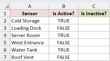
I want to return TRUE for inactive sensors and FALSE for active sensors.
Here is the formula:
=NOT(B2:B7)
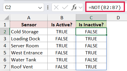
NOT reverses each value in B2:B7. The results spill from C2 to C7, so Loading Dock, West Entrance, and Roof Vent return TRUE in the Is Inactive? column.
You only enter the formula in C2. Excel fills the rest of the spill range automatically.
Example 2: Flag Values That Are Not Approved
Now let’s reverse the result of a text comparison.
Below is the dataset with seven permit numbers and their current review statuses.
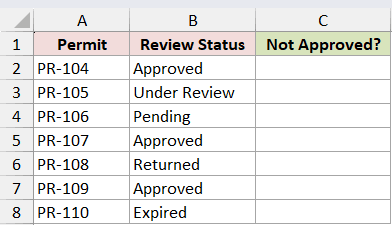
I want to flag every permit whose status is anything other than Approved.
Here is the formula:
=NOT(B2:B8="Approved")
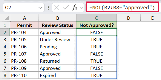
The expression B2:B8="Approved" returns TRUE for approved permits. NOT reverses those results, so Under Review, Pending, Returned, and Expired are flagged TRUE.
Pro Tip: For a simple text comparison, =B2:B8<>"Approved" is shorter. The does not equal operator returns the same spilled results, while NOT is useful when the test itself is more involved.
Example 3: Return an Action with IF and NOT
Here’s a practical way to nest NOT inside another logical formula.
Below is the dataset with seven fleet units and the number of days since each one was inspected.
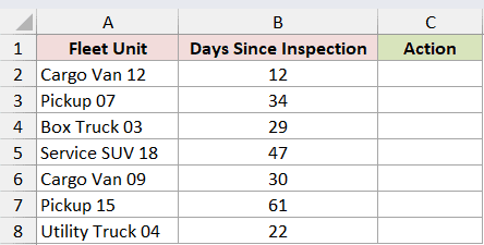
I want to schedule an inspection when a vehicle is not within the 30-day inspection window.
Here is the formula:
=IF(NOT(B2:B8<=30),"Schedule inspection","Current")
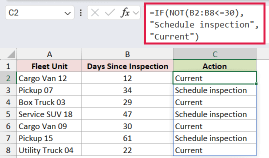
NOT reverses the B2:B8<=30 test. Values above 30 therefore become TRUE, and the IF function returns Schedule inspection for Pickup 07, Service SUV 18, and Pickup 15.
A value of exactly 30 remains Current because it satisfies the original less-than-or-equal-to test.
Example 4: Check Which Cells Are Not Blank
This example focuses on cells that are physically empty.
Below is the dataset with six pieces of equipment and their asset tags. Two asset-tag cells are empty.
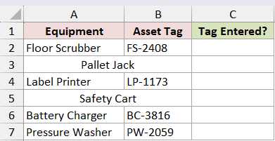
I want TRUE beside equipment that has an entered asset tag.
Here is the formula:
=NOT(ISBLANK(B2:B7))
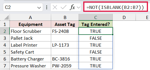
ISBLANK returns TRUE for the empty cells. NOT flips those results, so Pallet Jack and Safety Cart return FALSE while the four tagged items return TRUE.
Pro Tip: ISBLANK tests whether a cell is physically empty. If formulas that return an empty string should also count as blank, use =B2:B7<>"" to test for displayed content instead.
Example 5: Find Case-Sensitive Label Mismatches
Now let’s find label differences that a regular comparison can miss.
Below is the dataset with seven scanned package labels and the reference label expected for each package.
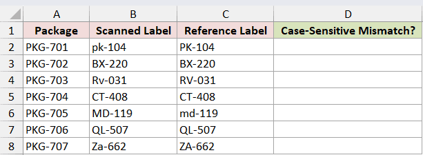
I want TRUE when the two labels differ, including differences in capitalization.
Here is the formula:
=NOT(EXACT(B2:B8,C2:C8))
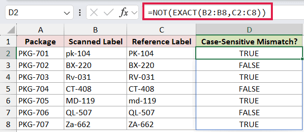
EXACT compares each text pair and returns TRUE only when the characters and capitalization match. NOT reverses that result, flagging PKG-701, PKG-703, PKG-705, and PKG-707.
The normal <> comparison is case-insensitive, so NOT with EXACT is the better choice when letter case matters.
Example 6: Filter Out Multiple Statuses
Finally, let’s use NOT to exclude more than one status from a report.
Below is the dataset with eight restaurant reservations, their statuses, and party sizes.
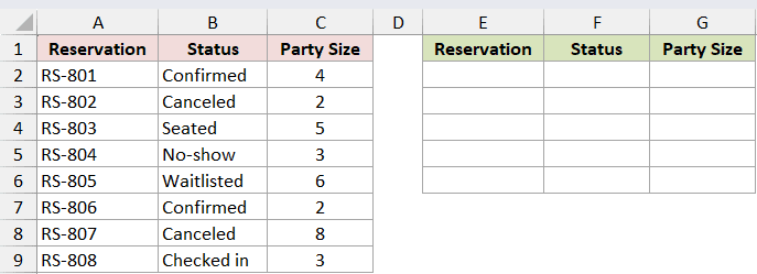
I want to return reservations whose status is neither Canceled nor No-show.
Here is the formula:
=FILTER(A2:C9,NOT(ISNUMBER(XMATCH(B2:B9,{"Canceled","No-show"}))),"No active reservations")
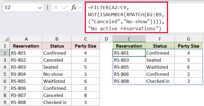
XMATCH searches for each status in the two-item exclusion list. ISNUMBER returns TRUE when it finds a match, and NOT reverses that to FALSE so FILTER removes that row.
The result contains five reservations: RS-801, RS-803, RS-805, RS-806, and RS-808.
Pro Tip: A cleaner modern include test is =FILTER(A2:C9,ISNA(XMATCH(B2:B9,{"Canceled","No-show"})),"No active reservations"). ISNA returns TRUE when XMATCH does not find an excluded status.
Tips & Common Mistakes
- NOT accepts one logical argument. Combine several tests inside AND or OR before passing the result to NOT.
- In Excel 365, a range passed to NOT returns a spilled array. In older Excel versions, use a row-level formula and fill it down.
- Make sure the spill range is empty before entering a range-based NOT formula, or Excel returns a #SPILL! error.
- Remember that NOT reverses the whole expression inside its parentheses. Check the original test first if the result seems backward.
- Use EXACT when a text mismatch must be case-sensitive. The standard equality and inequality operators ignore letter case.
I use NOT when the condition is easier to state in its positive form and then reverse. The examples above cover Boolean values, text tests, IF logic, blanks, case-sensitive comparisons, and filtered exclusions.
I hope you found this article helpful.
Related Excel Functions / Articles:
